Stochastic Optimization in R by Parallel Tempering


I’ve written a few posts now about using parallel tempering to sample from complicated multi-modal target distributions but there are also other benefits and uses to this algorithm. There is a nice post on Darren Wilkinson’s blog about using tempered posteriors for marginal likelihood calculations. There is also another area where parallel tempering finds application, namely in stochastic optimization. I first encountered parallel tempering whilst doing my MPhys degree at the University of Warwick but at that time it was employed as a stochastic optimization algorithm to find the minimum energy configuration of a Lennard-Jones cluster as opposed to a sampling algorithm. All that is required is one observation to turn this sampling algorithm into a stochastic optimization algorithm. Lets break this observation down into a few steps.
Consider sampling from a simple exponential distribution $$f(E)\propto e^{-\beta E}1_{(0,\infty )}(E),$$
with rate parameter beta. For now lets fix beta=5. One could sample from this distribution using the same Rmpi parallel tempering code given in my previous post by simply changing the target distribution to the exponential above. The histograms of mcmc draws from four tempered distribution would then look something like this:
Histogram of mcmc draws
Note the scale on the x-axis. The two important observations mentioned earlier are

  • The minimum value of E occurs most frequently as it the mode of the target distribution
  • The greater the rate parameter, the more concentrated the distribution is around E-min
  • The second point is important because although the sampling algorithm is creating draws that are not the minimum value of E, by increasing the rate parameter one can force these draws to be arbitrarily close to E-min.

    A Uni-modal Optimization Function

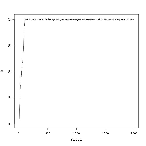
    How does this relate to optimization? Consider setting $$E(\theta)=(\theta-40)^2$$ Whereas before where using the Metropolis algorithm one would propose a new value of E, say E’, now the proposal is made in θ, and θ’ is accepted based on u < f(E(θ')) / f(E(θ)). By construction the algorithm gives draws close to E-min, which occurs when θ=40. The traceplot of θ is shown below: Stochastic Optimization mcmc traceplot
    Click here for the code.

    A Harder Optimization Function

    The above quadratic was an easy uni-modal example. Let’s try a harder function. Consider the minimum of $$ E(\theta)=3sin(\theta)+(0.1\theta-3)^2,$$ which looks like this:
    Optimization Function
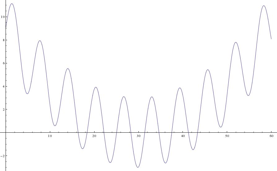
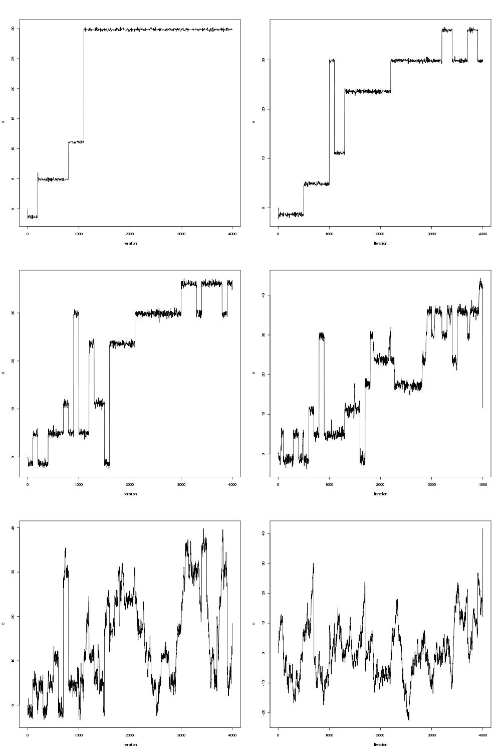
    This function has infinitely many local minima but one global minimum around 30. Local minima make optimization challenging and many optimization algorithms get stuck in these regions as locally it appears the minimum has been reached. This is where the parallel tempering really helps. The traceplots of theta are shown for six tempered distributions below:
    optimization traceplots mcmc
    Click here for the code.

    I’m currently working on another example just for fun, namely finding the lowest energy configuration of an n-particle Lennard-Jones cluster. This is a nice example because one can visualize the process using vmd and it also provides some insight into the origins of such terminology as “tempering”, “annealing” and “temperature” which always look somewhat out of place in the statistics literature.

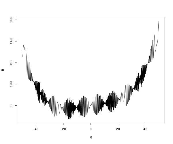
    An Even Harder Function

    Consider the function
    $$ E(\theta)=10\sin(0.3\theta)\sin(1.3\theta^2) + 0.00001\theta^4 + 0.2\theta+80, $$
    which is shown below.
    Optimization Function

    The trace-plots for the parallel tempering optimization are shown below
    Parallel Tempering Optimization

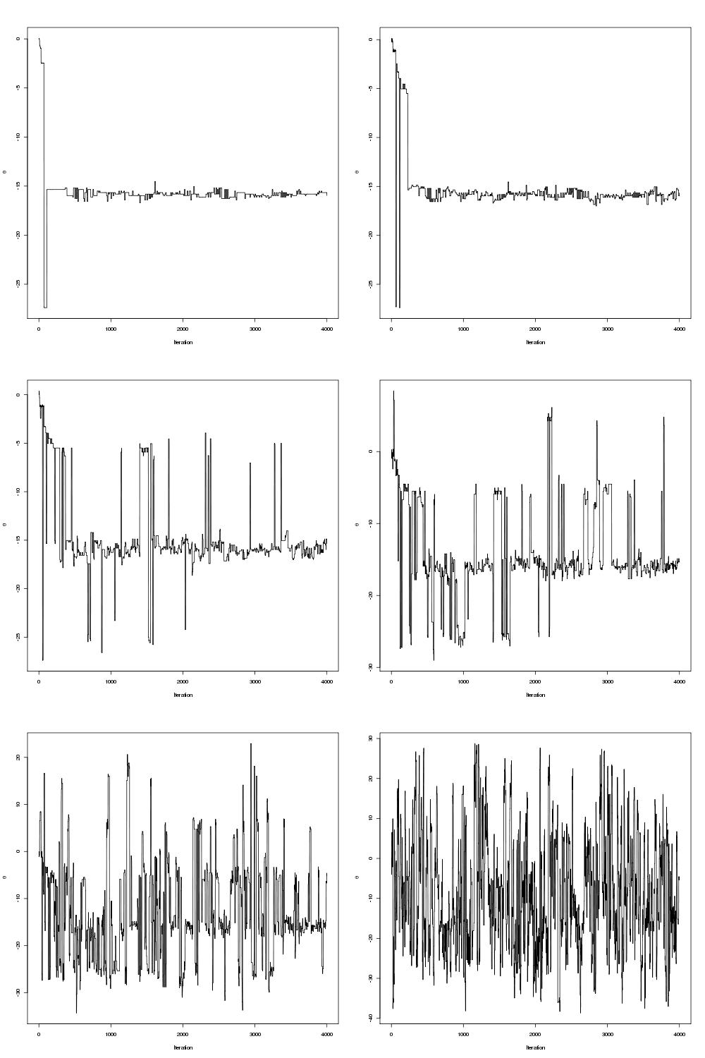
    Examining the mcmc draws the minimum is obtained at theta=-15.81515.

    Li Y., Protopopescu V.A., Arnold N., Zhang X. & Gorin A. (2009). Hybrid parallel tempering and simulated annealing method, Applied Mathematics and Computation, 212 (1) 216-228. DOI:

    • Genetic algorithms cracks this very fast:

      require(gaoptim)
      energy.inv = function(theta){-energy(theta)}
      ga = GAReal(energy.inv, -100, 100, selection = ‘uniform’)
      ga$evolve(100)
      print(ga$bestIndividual())

      Nice job anyway!

      • admin

        I gave your package a try and I have also uploaded the parallel tempering optimization results for your test (“Wild”) function. I don’t have much experience with genetic algorithms, how well do these genetic algorithms perform in higher dimensional spaces? Do they have any shortcomings?

        • I’m not a expert either, stochastic optimization is natural to understand but very hard to describe the math behind. Sometimes is very hard to design a fitness function, and there’s no guarantee of convergence, limiting the use in real time applications. If the search space is very very large, then it get’s worse. For example, the GA technique is probably fail to solve the Runge function polynomial approximation:

          # ga fail (answer is a minimum maximal abs deviation of around 0.06)
          require(pracma)
          n = 10
          m = 101
          xi = seq(-1, 1, length = m)
          yi <- 1 / (1 + (5*xi)^2)
          pfn <- function(p) max(abs(polyval(c(p), xi) – yi))

          But there's always a better choice i guess!

          • admin

            Hi Fernando, I can’t get this piece of code as it is here to run – is it missing something? Would you mind posting it again? Parallel tempering does have some issues, specifically the devil is in the details with tuning parameters such as the choice of temperature set and also how large the proposed moves are within each tempered distribution. That being said there are adaptive ideas out there which adjust the proposal size so that you get an acceptance rate of around 40% within each distribution and also rules of thumb about how to choose the temperatures (i.e. geometric). I’m keen to learn about other methods though, so if these genetic algorithms perform well I’ll take a look at them 🙂

    • Sure. The problem above is to approximate the function y = 1 / (1 + (5*xi)^2) using a polynomial of degree n. Using n = 10:

      require(gaoptim)
      require(pracma)

      n <- 10 # polynomial of degree 10
      m <- 101 # no. of data points
      xi <- seq(-1, 1, length = m)
      yi <- 1 / (1 + (5*xi)^2)

      pfn <- function(p) max(abs(polyval(c(p), xi) – yi))
      pfninv <- function(p){ 1/pfn(p) }

      ## set up a matrix for the polynomial data
      ndeg <- 10
      ndim <- ndeg + 1
      ga = GAReal(pfninv, lb = rep(-1000, ndim), ub = rep(1000, ndim), selection = 'uniform')

      ga$evolve(200)
      print(ga)

      You can use least squares and compare with a GA solution. I received a paper on this, i can send you, just need the email.

    • You can ask for the paper here:
      nashjc( at )uottawa( dot)ca

    • Raymond

      I read thro this and gone back to your earlier R mpi post,
      Sorry, still not sure how to ‘spread’ R process 2 PC (you got cabbage and lettuce).
      Shall I just run mpi.bcast…something, it will automatically bcast to all nodes but when did you define the nodes that are avaliable?