MALA – Metropolis Adjusted Langevin Algorithm in Julia

Metropolis Adjusted Langevin Algorithm (MALA)

Haven’t dumped much code here in a while. Here’s a Julia implementation of MALA with an arbitrary preconditioning matrix M. Potentially I might use this in the future.

Generic Julia Implementation

Arguments are a function to evaluate the logdensity, function to evaluate the gradient, a step size h, a preconditioning matrix M, number of iterations and an initial parameter value.

function mala(logdensity,gradient,h,M,niter,θinit)                                                                                                                                                                 
        function gradientStep(θ,t)                                                                                                                                                                                 
                θ-t*M*gradient(θ)                                                                                                                                                                                  
        end                                                                                                                                                                                                        
        θtrace=Array{Float64}(length(θinit),niter)                                                                                                                                                                 
        θ=θinit                                                                                                                                                                                                    
        θtrace[:,1]=θinit                                                                                                                                                                                          
        for i=2:niter                                                                                                                                                                                              
                θold=θ                                                                                                                                                                                             
                θ=rand(MvNormal(gradientStep(θ,0.5*h),h*M))                                                                                                                                                        
                d=logdensity(θ) - logdensity(θold) + logpdf(MvNormal(gradientStep(θ,0.5*h),h*M),θold) - logpdf(MvNormal(gradientStep(θold,0.5*h),h*M),θ)                                                           
                if(!(log(rand(Uniform(0,1)))<d))                                                                                                                                                                   
                        θ=θold                                                                                                                                                                                     
                end                                                                                                                                                                                                
                θtrace[:,i]=θ                                                                                                                                                                                      
        end                                                                                                                                                                                                        
        θtrace                                                                                                                                                                                                     
end     

Don’t forget to use the Distributions package of Julia.

Bivariate Normal Example

Consider a Bivariate Normal as an example

ρ²=0.8                                                                                                                                                                                                             
Σ=[1 ρ²;ρ² 1]                                                                                                                                                                                                      
                                                                                                                                                                                                                   
function logdensity(θ)                                                                                                                                                                                             
        logpdf(MvNormal(Σ),θ)                                                                                                                                                                                      
end                                                                                                                                                                                                                
                                                                                                                                                                                                                   
function gradient(θ)                                                                                                                                                                                               
        Σ\θ                                                                                                                                                                                                        
end   

and now the code to generate the plots and results

niter=1000                                                                                                                                                                                                         
h=1/eigs(inv(Σ),nev=1)[1][1]                                                                                                                                                                                       
@time draws=mala(logdensity,gradient,h,eye(2),niter,[5,50]);                                                                                                                                                       
sum(map(t -> draws[:,t]!=draws[:,t-1],2:niter))/(niter-1)                                                                                                                                                          
@time pdraws=mala(logdensity,gradient,h,Σ,niter,[5,50]);                                                                                                                                                           
sum(map(t -> pdraws[:,t]!=pdraws[:,t-1],2:niter))/(niter-1)                                                                                                                                                        
                                                                                                                                                                                                                   
function logdensity2d(x,y)                                                                                                                                                                                         
        logdensity([x,y])                                                                                                                                                                                          
end                                                                                                                                                                                                                
x = -30:0.1:30                                                                                                                                                                                                     
y = -30:0.1:50                                                                                                                                                                                                     
X = repmat(x',length(y),1)                                                                                                                                                                                         
Y = repmat(y,1,length(x))                                                                                                                                                                                          
Z = map(logdensity2d,Y,X)                                                                                                                                                                                          
p1 = contour(x,y,Z,200)                                                                                                                                                                                            
plot(vec(draws[1,:]),vec(draws[2,:]))                                                                                                                                                                              
plot(vec(pdraws[1,:]),vec(pdraws[2,:])) 

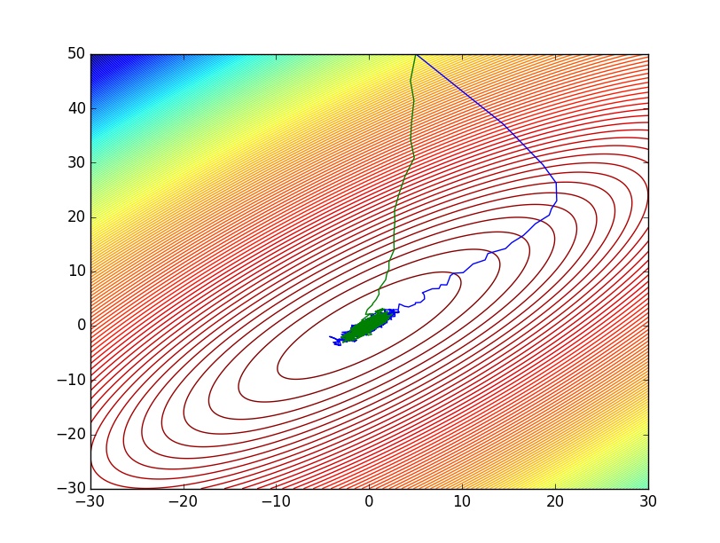
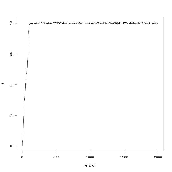
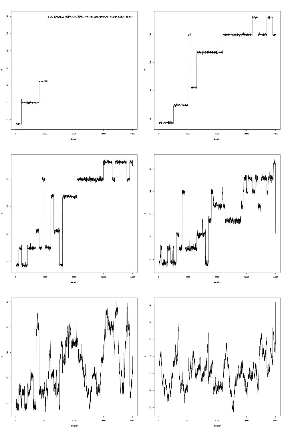
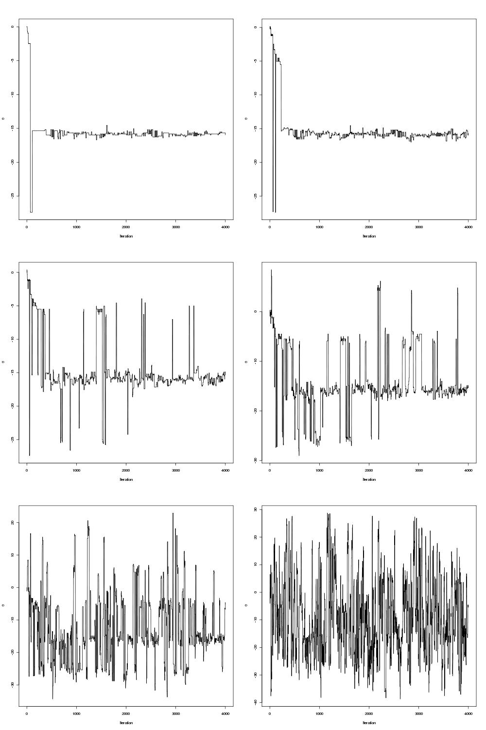
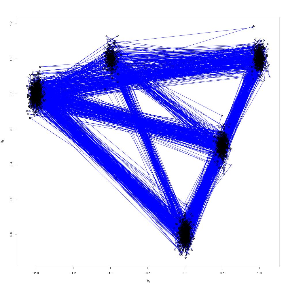
pdraws uses the covariance matrix Σ as the preconditioning matrix, whereas the first uses an identity matrix, resulting in the original MALA algorithm. The traceplot of draws from MALA and preconditioned MALA are shown in blue and green respectively…

mala

Traceplots for MALA and preconditioned MALA

Effective Sample Sizes in R

We can use the julia “RCall” package to switch over to R and use the coda library to evaluate the minimum effective sample size for both of these MCMC algorithms.

julia> library(coda)

R> library(coda)

R> min(effectiveSize($(draws')))
[1] 22.02418

R> min(effectiveSize($(pdraws')))
[1] 50.85163

I didn’t tune the step size h in this example at all (you should).

Generate Random Inverse Gaussian in R

Needed to generate draws from an inverse Gaussian today, so I wrote the following Rcpp code:

#include <RcppArmadillo.h>
// [[Rcpp::depends(RcppArmadillo)]]

using namespace Rcpp;
using namespace arma;

// [[Rcpp::export]]
Col<double> rrinvgauss(int n, double mu, double lambda){

	Col<double> random_vector(n);
	double z,y,x,u;

	for(int i=0; i<n; ++i){
		z=R::rnorm(0,1);
		y=z*z;
		x=mu+0.5*mu*mu*y/lambda - 0.5*(mu/lambda)*sqrt(4*mu*lambda*y+mu*mu*y*y);
		u=R::runif(0,1);
		if(u <= mu/(mu+x)){
			random_vector(i)=x;
		}else{
			random_vector(i)=mu*mu/x;
		};
	}
	return(random_vector);
}

It seems to be faster than existing implementations such as rig from mgcv and rinvgauss from statmod packages.

library(Rcpp) 
library(RcppArmadillo)
library(rbenchmark)
library(statmod)
library(mgcv)
sourceCpp("rrinvgauss.cpp")
n=10000 
benchmark(rig(n,1,1),rinvgauss(n,1,1),rrinvgauss(n,1,1),replications=100)

inverse gaussian

rename rrinvgauss as desired.

Generalized Double Pareto Priors for Regression

This post is a review of the “GENERALIZED DOUBLE PARETO SHRINKAGE” Statistica Sinica (2012) paper by Armagan, Dunson and Lee.

Consider the regression model \(Y=X\beta+\varepsilon\) where we put a generalized double pareto distribution as the prior on the regression coefficients \(\beta\). The GDP distribution has density
$$\begin{equation}
f(\beta|\xi,\alpha)=\frac{1}{2\xi}\left( 1+\frac{|\beta|}{\alpha\xi} \right)^{-(\alpha+1)}.
\label{}
\end{equation}$$

GDP as Scale Mixture of Normals

The GDP distribution can be conveniently represented as a scale mixture of normals. Let
$$\begin{align*}
\beta_{i}|\phi,\tau_{i} &\sim N(0,\phi^{-1}\tau_{i})\\
\tau_{i}|\lambda_{i}&\sim Exp(\frac{\lambda_{i}^{2}}{2})\\
\lambda_{i}&\sim Ga(\alpha,\eta)\\
\end{align*}$$
then \(\beta|\phi \sim GDP(\xi=\frac{\eta}{\sqrt{\phi}\alpha},\alpha)\).
To see this first note that \(\beta_{i}|\phi,\lambda_{i}\) has a Laplace or Double Exponential distribution with rate parameter \(\sqrt{\phi}\lambda_{i}\).
$$\begin{align*}
p(\beta_{i}|\phi,\lambda_{i})&=\int p(\beta_{i}|\phi,\tau_{i})p(\tau_{i}|\lambda_{i})d\tau_{i}\\
\psi(t)&=\int e^{it\beta_{i}} \int p(\beta_{i}|\phi,\tau_{i})p(\tau_{i}|\lambda_{i})d\tau_{i} d\beta_{i}\\
&=\int \int e^{it\beta_{i}}p(\beta_{i}|\phi,\tau_{i})d\beta_{i}p(\tau_{i}|\lambda_{i})d\tau_{i}\\
&=\int e^{-\frac{1}{2}\frac{\tau_{i}}{\phi}t^{2}}p(\tau_{i}|\lambda_{i})d\tau_{i}\\
&=\frac{\lambda_{i}^{2}}{2} \int e^{-\frac{1}{2}(\frac{t^{2}}{\phi}+\frac{\lambda_{i}^{2}}{2})\tau_{i}}d\tau_{i}\\
&=\frac{\phi\lambda_{i}^{2}}{t^{2}+\phi\lambda_{i}^{2}},
\end{align*}$$
which is the characteristic function of a Double Exponential distribution with rate parameter \(\sqrt{\phi}\lambda_{i}\).
Lastly
$$\begin{align*}
p(\beta_{i}|\phi)&=\int p(\beta_{i}|\phi,\lambda_{i})p(\lambda_{i})d\lambda_{i}\\
&=\frac{1}{2}\sqrt{\phi}\frac{\eta^{\alpha}}{\Gamma(\alpha)}\frac{\Gamma(\alpha+1)}{(\eta+\sqrt{\phi}|\beta_{i}|)^{\alpha+1}}\\
&=\frac{1}{2}\frac{\sqrt{\phi}\alpha}{\eta}\left( 1+\frac{\sqrt{\phi}\alpha}{\eta}\frac{|\beta_{i}|}{\alpha} \right)^{-(\alpha+1)},
\end{align*}$$
which is the density of a \(GDP(\xi=\frac{\eta}{\sqrt{\phi}\alpha},\alpha)\).

EM Algorithm

\(\tau_{i}\) and \(\lambda_{i}\) are treated as missing data for each \(i\).
\begin{align*}
Q(\beta,\phi||\beta^{(t)},\phi^{(t)})&=c+\mathbb{E}_{\tau,\lambda}\left[ \log p(\beta,\phi|Y,\tau,\lambda)|\beta^{(t)},\phi^{(t)} \right]\\
&=\frac{n+p-3}{2}\log\phi – \frac{\phi}{2}||Y-X\beta||^{2}-\frac{\phi}{2}\sum_{i=1}^{p}\beta_{i}^{2}\mathbb{E}\left[ \frac{1}{\tau_{i}} \right]\\
\end{align*}

Expectation

For the iterated expectation one needs the distribution \(\tau_{i}|\lambda_{i},\beta_{i},\phi\) and \(\lambda_{i}|\beta_{i},\phi\).
\begin{align*}
p(\tau_{i}|\beta_{i},\lambda_{i},\phi)&\propto p(\beta_{i}|\phi,\tau_{i})p(\tau_{i}|\lambda_{i})\\
&\propto \left( \frac{1}{\tau_{i}} \right)^{\frac{1}{2}}e^{-\frac{1}{2}(\frac{\phi \beta_{i}^{2}}{\tau_{i}}+\lambda_{i}^{2}\tau_{i})}
\end{align*}
This is the kernel of a Generalized Inverse Gaussian distribution, specifically \(p(\tau_{i}|\beta_{i},\lambda_{i},\phi)=GIG(\tau_{i}:\lambda_{i}^{2},\phi \beta_{i}^{2},\frac{1}{2})\).
By a standard change of variables it follows that \(p(\frac{1}{\tau_{i}}|\beta_{i},\lambda_{i},\phi)=IG(\frac{1}{\tau_{i}}:\sqrt{\frac{\lambda_{i}^{2}}{\phi \beta_{i}^{2}}},\lambda_{i}^{2})\) and so \(\mathbb{E}\left[ \frac{1}{\tau_{i}}|\lambda_{i},\beta^{(t)},\phi^{(t)} \right]=\frac{\lambda_{i}}{\sqrt{\phi^{(t)}}|\beta_{i}^{(t)}|}\).

Recall that \(p(\beta_{i}|\phi,\lambda_{i})\) has a double exponential distribution with rate \(\sqrt{\phi}\lambda_{i}\).
Hence from \(p(\lambda_{i}|\beta_{i},\phi)\propto p(\beta_{i}|\lambda_{i},\phi)p(\lambda_{i})\) it follows that \(\lambda_{i}|\beta_{i},\phi \sim Ga(\alpha+1,\eta+\sqrt{\phi}|\beta_{i}|)\), then performing the expectation with respect to \(\lambda_{i}\) yields
\begin{align*}
\mathbb{E}\left[ \frac{1}{\tau_{i}}|\beta^{(t)},\phi^{(t)} \right]=\left( \frac{\alpha+1}{\eta+\sqrt{\phi^{t}}|\beta_{i}^{(t)}|} \right)\left( \frac{1}{\sqrt{\phi^{(t)}}|\beta_{i}^{(t)}|} \right)
\end{align*}

Maximization

Writing \(D^{(t)}=diag(\mathbb{E}[\frac{1}{\tau_{1}}],\dots,\mathbb{E}[\frac{1}{\tau_{p}}])\) the function to maximize is
\begin{align*}
Q(\beta,\phi||\beta^{(t)},\phi^{(t)})&=c+\mathbb{E}_{\tau,\lambda}\left[ \log p(\beta,\phi|Y,\tau,\lambda)|\beta^{(t)},\phi^{(t)} \right]\\
&=\frac{n+p-3}{2}\log\phi – \frac{\phi}{2}||Y-X\beta||^{2}-\frac{\phi}{2}\beta^{‘}D^{(t)}\beta,\\
\end{align*}
which is maximized by letting
\begin{align*}
\beta^{(t+1)}&=(X^{‘}X+D^{(t)})^{-1}X^{‘}Y\\
\phi^{(t+1)}&=\frac{n+p-3}{Y^{‘}(I-X(X^{‘}X+D^{(t)})^{-1}X^{‘})Y}\\
&=\frac{n+p-3}{||Y-X\beta^{(t+1)}||^{2}+\beta^{(t+1)’}D^(t)\beta^{(t+1)}}\\
\end{align*}

R CPP Code

#include <RcppArmadillo.h>
// [[Rcpp::depends(RcppArmadillo)]]

using namespace Rcpp;
using namespace arma;

double gdp_log_posterior_density(int no, int p, double alpha, double eta, const Col<double>& yo, const Mat<double>& xo, const Col<double>& B,double phi);

// [[Rcpp::export]]
List gdp_em(NumericVector ryo, NumericMatrix rxo, SEXP ralpha, SEXP reta){

	//Define Variables//
	int p=rxo.ncol();
	int no=rxo.nrow();
	double eta=Rcpp::as<double >(reta);
	double alpha=Rcpp::as<double >(ralpha);

	//Create Data//
	arma::mat xo(rxo.begin(), no, p, false);
	arma::colvec yo(ryo.begin(), ryo.size(), false);
	yo-=mean(yo);

	//Pre-Processing//
	Col<double> xoyo=xo.t()*yo;
	Col<double> B=xoyo/no;
	Col<double> Babs=abs(B);
	Mat<double> xoxo=xo.t()*xo;
	Mat<double> D=eye(p,p);
	Mat<double> Ip=eye(p,p);
	double yoyo=dot(yo,yo);
	double deltaB;
	double deltaphi;
	double phi=no/dot(yo-xo*B,yo-xo*B);
	double lp;

	//Create Trace Matrices
	Mat<double> B_trace(p,20000);
	Col<double> phi_trace(20000);
	Col<double> lpd_trace(20000);

	//Run EM Algorithm//
	cout << "Beginning EM Algorithm" << endl;
	int t=0;
	B_trace.col(t)=B;
	phi_trace(t)=phi;
	lpd_trace(t)=gdp_log_posterior_density(no,p,alpha,eta,yo,xo,B,phi);
	do{
		t=t+1;


		Babs=abs(B);
		D=diagmat(sqrt(((eta+sqrt(phi)*Babs)%(sqrt(phi)*Babs))/(alpha+1)));
		B=D*solve(D*xoxo*D+Ip,D*xoyo);

		phi=(no+p-3)/(yoyo-dot(xoyo,B));

		//Store Values//
		B_trace.col(t)=B;
		phi_trace(t)=phi;
		lpd_trace(t)=gdp_log_posterior_density(no,p,alpha,eta,yo,xo,B,phi);

		deltaB=dot(B_trace.col(t)-B_trace.col(t-1),B_trace.col(t)-B_trace.col(t-1));
		deltaphi=phi_trace(t)-phi_trace(t-1);
	} while((deltaB>0.00001 || deltaphi>0.00001) && t<19999);
	cout << "EM Algorithm Converged in " << t << " Iterations" << endl;

	//Resize Trace Matrices//
	B_trace.resize(p,t);
	phi_trace.resize(t);
	lpd_trace.resize(t);

	return Rcpp::List::create(
			Rcpp::Named("B") = B,
			Rcpp::Named("B_trace") = B_trace,
			Rcpp::Named("phi") = phi,
			Rcpp::Named("phi_trace") = phi_trace,
			Rcpp::Named("lpd_trace") = lpd_trace
			) ;

}


double gdp_log_posterior_density(int no, int p, double alpha, double eta, const Col<double>& yo, const Mat<double>& xo, const Col<double>& B,double phi){

	double lpd;
	double xi=eta/(sqrt(phi)*alpha);
	lpd=(double)0.5*((double)no-1)*log(phi/(2*M_PI))-p*log(2*xi)-(alpha+1)*sum(log(1+abs(B)/(alpha*xi)))-0.5*phi*dot(yo-xo*B,yo-xo*B)-log(phi);
	return(lpd);

}

An Example in R

rm(list=ls())
library(Rcpp)
library(RcppArmadillo)
sourceCpp("src/gdp_em.cpp")

#Generate Design Matrix
set.seed(3)
no=100
foo=rnorm(no,0,1)
sd=4
xo=cbind(foo+rnorm(no,0,sd),foo+rnorm(no,0,sd),foo+rnorm(no,0,sd),foo+rnorm(no,0,sd),foo+rnorm(no,0,sd),foo+rnorm(no,0,sd),foo+rnorm(no,0,sd),foo+rnorm(no,0,sd))
for(i in 1:40) xo=cbind(xo,foo+rnorm(no,0,sd),foo+rnorm(no,0,sd),foo+rnorm(no,0,sd),foo+rnorm(no,0,sd),foo+rnorm(no,0,sd),foo+rnorm(no,0,sd),foo+rnorm(no,0,sd))

#Scale and Center Design Matrix
xo=scale(xo,center=T,scale=F)
var=apply(xo^2,2,sum)
xo=scale(xo,center=F,scale=sqrt(var/no))

#Generate Data under True Model
p=dim(xo)[2]
b=rep(0,p)
b[1]=1
b[2]=2
b[3]=3
b[4]=4
b[5]=5
xo%*%b
yo=xo%*%b+rnorm(no,0,1)
yo=yo-mean(yo)

#Run GDP
gdp=gdp_em(yo,xo,100,100)

#Posterior Density Increasing at Every Iteration?
gdp$lpd_trace[2:dim(gdp$lpd_trace)[1],1]-gdp$lpd_trace[1:(dim(gdp$lpd_trace)[1]-1),1]>=0
mean(gdp$lpd_trace[2:dim(gdp$lpd_trace)[1],1]-gdp$lpd_trace[1:(dim(gdp$lpd_trace)[1]-1),1]>=0)

#Plot Results
plot(gdp$B,ylab=expression(beta[GDP]),main="GDP MAP Estimate of Regression Coefficients")

Generalized Double Pareto Estimated Coefficients

WEST M. (1987). On scale mixtures of normal distributions, Biometrika, 74 (3) 646-648. DOI: http://dx.doi.org/10.1093/biomet/74.3.646

Artin Armagan, David Dunson, & Jaeyong Lee (2011). Generalized double Pareto shrinkage Statistica Sinica 23 (2013), 119-143 arXiv: 1104.0861v4

Figueiredo M.A.T. (2003). Adaptive sparseness for supervised learning, IEEE Transactions on Pattern Analysis and Machine Intelligence, 25 (9) 1150-1159. DOI: http://dx.doi.org/10.1109/tpami.2003.1227989

Also see this similar post on the Bayesian lasso.

EM Algorithm for Bayesian Lasso R Cpp Code

Bayesian Lasso

$$\begin{align*}
p(Y_{o}|\beta,\phi)&=N(Y_{o}|1\alpha+X_{o}\beta,\phi^{-1} I_{n{o}})\\
\pi(\beta_{i}|\phi,\tau_{i}^{2})&=N(\beta_{i}|0, \phi^{-1}\tau_{i}^{2})\\
\pi(\tau_{i}^{2})&=Exp \left( \frac{\lambda}{2} \right)\\
\pi(\phi)&\propto \phi^{-1}\\
\pi(\alpha)&\propto 1\\
\end{align*}$$

Marginalizing over \(\alpha\) equates to centering the observations and losing a degree of freedom and working with the centered \( Y_{o} \).
Mixing over \(\tau_{i}^{2}\) leads to a Laplace or Double Exponential prior on \(\beta_{i}\) with rate parameter \(\sqrt{\phi\lambda}\) as seen by considering the characteristic function
$$\begin{align*}
\varphi_{\beta_{i}|\phi}(t)&=\int e^{jt\beta_{i}}\pi(\beta_{i}|\phi)d\beta_{i}\\
&=\int \int e^{jt\beta_{i}}\pi(\beta_{i}|\phi,\tau_{i}^{2})\pi(\tau_{i}^{2})d\tau_{i} d\beta_{i}\\
&=\frac{\lambda}{2} \int e^{-\frac{1}{2}\frac{t^{2}}{\phi}\tau_{i}^{2}}e^{-\frac{\lambda}{2}\tau_{i}^{2}}d\tau_{i}\\
&=\frac{\lambda}{\frac{t^{2}}{\phi}+\lambda}=\frac{\lambda\phi}{t^{2}+\lambda\phi}
\end{align*}$$.

EM Algorithm

The objective is to find the mode of the joint posterior \(\pi(\beta,\phi|Y_{o})\). It is easier, however, to find the joint mode of \(\pi(\beta,\phi|Y_{o},\tau^{2})\) and use EM to exploit the scale mixture representation.

$$\begin{align*}
\log \pi(\beta,\phi|Y_{o},\tau^{2})=c+ \frac{n_o+p-3}{2}\log \phi -\frac{\phi}{2}||Y_{o}-X_{o}\beta||^{2}-\sum_{i=1}^{p}\frac{\phi}{2}\frac{1}{\tau_{i}^{2}}\beta^{2}_{i}
\end{align*}$$

Expectation

The expecation w.r.t. \(\tau_{i}^{2}\) is handled as by
$$
\begin{align*}
&\frac{\lambda}{2}\int \frac{1}{\tau_{i}^{2}}\left( \frac{\phi}{2\pi\tau_{i}^{2}} \right)^{\frac{1}{2}}e^{-\frac{1}{2}\phi\beta_{i}^{2}\frac{1}{\tau_{i}^{2}}}e^{-\frac{\lambda}{2}\tau_{i}^{2}}d\tau_{i}^{2}\\
&\frac{\lambda}{2}\int \left( \frac{\phi}{2\pi[\tau_{i}^{2}]^{3}} \right)^{\frac{1}{2}}e^{-\frac{1}{2}\phi\beta_{i}^{2}\frac{1}{\tau_{i}^{2}}}e^{-\frac{\lambda}{2}\tau_{i}^{2}}d\tau_{i}^{2}\\
\end{align*}$$

This has the kernel of an Inverse Gaussian distribution with shape parameter \(\phi \beta_{i}^{2}\) and mean \(\sqrt{\frac{\phi}{\lambda}}|\beta_{i}|\)

$$\begin{align*}
&\frac{{\lambda}}{2|\beta_{i}|}\int \left( \frac{\beta_{i}^{2}\phi}{2\pi[\tau_{i}^{2}]^{3}} \right)^{\frac{1}{2}}e^{-\frac{1}{2}\phi\beta_{i}^{2}\frac{1}{\tau_{i}^{2}}}e^{-\frac{\lambda}{2}\tau_{i}^{2}}d\tau_{i}^{2}\\
&\frac{\lambda}{2|\beta_{i}|}e^{-\sqrt{\lambda\phi\beta_{i}^{2}}}\int \left( \frac{\beta_{i}^{2}\phi}{2\pi[\tau_{i}^{2}]^{3}} \right)^{\frac{1}{2}}e^{-\frac{1}{2}\phi\beta_{i}^{2}\frac{1}{\tau_{i}^{2}}}e^{-\frac{\lambda}{2}\tau_{i}^{2}}e^{\sqrt{\lambda\phi\beta_{i}^{2}}}d\tau_{i}^{2}\\
&\frac{\lambda}{2|\beta_{i}|}e^{-\sqrt{\lambda\phi\beta_{i}^{2}}}\\
\end{align*}$$

Normalization as follows

$$\begin{align*}
&\frac{\lambda}{2}\int \left( \frac{\phi}{2\pi\tau_{i}^{2}} \right)^{\frac{1}{2}}e^{-\frac{1}{2}\phi\beta_{i}^{2}\frac{1}{\tau_{i}^{2}}}e^{-\frac{\lambda}{2}\tau_{i}^{2}}d\tau_{i}^{2}\\
&\frac{\lambda}{2}\int \tau_{i}^{2}\left( \frac{\phi}{2\pi[\tau_{i}^{2}]^{3}} \right)^{\frac{1}{2}}e^{-\frac{1}{2}\phi\beta_{i}^{2}\frac{1}{\tau_{i}^{2}}}e^{-\frac{\lambda}{2}\tau_{i}^{2}}d\tau_{i}^{2}\\
\end{align*}$$
$$\begin{align*}
&\frac{\lambda}{2|\beta_{i}|}e^{-\sqrt{\lambda\phi\beta_{i}^{2}}}\sqrt{\frac{\phi}{\lambda}}|\beta_{i}|\\
\end{align*}$$

\( \Rightarrow \mathbb{E}\left[ \frac{1}{\tau_{i}^{2}} \right]=\sqrt{\frac{\lambda}{\phi^{t}}}\frac{1}{|\beta_{i}^{t}|}\).
Let \(\Lambda^{t}=diag(\sqrt{\frac{\lambda}{\phi^{t}}}\frac{1}{|\beta_{1}^{t}|}, \dots, \sqrt{\frac{\lambda}{\phi^{t}}}\frac{1}{|\beta_{p}^{t}|})\).

Maximization

$$\begin{align*}
&Q(\beta,\phi||\beta^{t},\phi^{t})=c+ \frac{n_o+p-3}{2}\log \phi -\frac{\phi}{2}||Y_{o}-X_{o}\beta||^{2} – \frac{\phi}{2}\beta^{T}\Lambda^{t}\beta\\
&=c+ \frac{n_o+p-3}{2}\log \phi -\frac{\phi}{2}||\beta-(X_{o}^{T}X_{o}+\Lambda^{t})^{-1}X_{o}^{T}Y_{o}||^{2}_{(X_{o}^{T}X_{o}+\Lambda^{t})}-\frac{\phi}{2}Y_{o}^{T}(I_{n_{o}}-X_{o}^{T}(X_{o}^{T}X_{o}+\Lambda^{t})^{-1}X_{o})Y_{o}\\
\end{align*}$$

$$\begin{align*}
\beta^{t+1}&=(X_{o}^{T}X_{o}+\Lambda^{t})^{-1}X_{o}^{T}Y_{o}\\
\end{align*}$$

$$\begin{align*}
\phi^{t+1}=\frac{n_{o}+p-3}{Y_{o}^{T}(I_{n_{o}}-X_{o}^{T}(X_{o}^{T}X_{o}+\Lambda^{t})^{-1}X_{o})Y_{o}}
\end{align*}$$

RCpp C++ Code

#include <RcppArmadillo.h>
// [[Rcpp::depends(RcppArmadillo)]]

using namespace Rcpp;
using namespace arma;

double or_log_posterior_density(int no, int p, double lasso, const Col<double>& yo, const Mat<double>& xo, const Col<double>& B,double phi);

// [[Rcpp::export]]
List or_lasso_em(NumericVector ryo, NumericMatrix rxo, SEXP rlasso){

	//Define Variables//
	int p=rxo.ncol();
	int no=rxo.nrow();
	double lasso=Rcpp::as<double >(rlasso);

	//Create Data//
	arma::mat xo(rxo.begin(), no, p, false);
	arma::colvec yo(ryo.begin(), ryo.size(), false);
	yo-=mean(yo);

	//Pre-Processing//
	Col<double> xoyo=xo.t()*yo;
	Col<double> B=xoyo/no;
	Col<double> Babs=abs(B);
	Mat<double> xoxo=xo.t()*xo;
	Mat<double> D=eye(p,p);
	Mat<double> Ip=eye(p,p);
	double yoyo=dot(yo,yo);
	double deltaB;
	double deltaphi;
	double phi=no/dot(yo-xo*B,yo-xo*B);
	double lp;

	//Create Trace Matrices
	Mat<double> B_trace(p,20000);
	Col<double> phi_trace(20000);
	Col<double> lpd_trace(20000);

	//Run EM Algorithm//
	cout << "Beginning EM Algorithm" << endl;
	int t=0;
	B_trace.col(t)=B;
	phi_trace(t)=phi;
	lpd_trace(t)=or_log_posterior_density(no,p,lasso,yo,xo,B,phi);
	do{
		t=t+1;

		lp=sqrt(lasso/phi);

		Babs=abs(B);
		D=diagmat(sqrt(Babs));
		B=D*solve(D*xoxo*D+lp*Ip,D*xoyo);

		phi=(no+p-3)/(yoyo-dot(xoyo,B));

		//Store Values//
		B_trace.col(t)=B;
		phi_trace(t)=phi;
		lpd_trace(t)=or_log_posterior_density(no,p,lasso,yo,xo,B,phi);

		deltaB=dot(B_trace.col(t)-B_trace.col(t-1),B_trace.col(t)-B_trace.col(t-1));
		deltaphi=phi_trace(t)-phi_trace(t-1);
	} while((deltaB>0.00001 || deltaphi>0.00001) && t<19999);
	cout << "EM Algorithm Converged in " << t << " Iterations" << endl;

	//Resize Trace Matrices//
	B_trace.resize(p,t);
	phi_trace.resize(t);
	lpd_trace.resize(t);

	return Rcpp::List::create(
			Rcpp::Named("B") = B,
			Rcpp::Named("B_trace") = B_trace,
			Rcpp::Named("phi") = phi,
			Rcpp::Named("phi_trace") = phi_trace,
			Rcpp::Named("lpd_trace") = lpd_trace
			) ;

}


double or_log_posterior_density(int no, int p, double lasso, const Col<double>& yo, const Mat<double>& xo, const Col<double>& B,double phi){

	double lpd;
	lpd=(double)0.5*((double)no-1)*log(phi/(2*M_PI))-0.5*phi*dot(yo-xo*B,yo-xo*B)+0.5*(double)p*log(phi*lasso)-sqrt(phi*lasso)*sum(abs(B))-log(phi);
	return(lpd);

}

An Example in R

rm(list=ls())

#Generate Design Matrix
set.seed(3)
no=100
foo=rnorm(no,0,1)
sd=4
xo=cbind(foo+rnorm(no,0,sd),foo+rnorm(no,0,sd),foo+rnorm(no,0,sd),foo+rnorm(no,0,sd),foo+rnorm(no,0,sd),foo+rnorm(no,0,sd),foo+rnorm(no,0,sd),foo+rnorm(no,0,sd))
for(i in 1:40) xo=cbind(xo,foo+rnorm(no,0,sd),foo+rnorm(no,0,sd),foo+rnorm(no,0,sd),foo+rnorm(no,0,sd),foo+rnorm(no,0,sd),foo+rnorm(no,0,sd),foo+rnorm(no,0,sd))

#Scale and Center Design Matrix
xo=scale(xo,center=T,scale=F)
var=apply(xo^2,2,sum)
xo=scale(xo,center=F,scale=sqrt(var/no))

#Generate Data under True Model
p=dim(xo)[2]
b=rep(0,p)
b[1]=1
b[2]=2
b[3]=3
b[4]=4
b[5]=5
xo%*%b
yo=xo%*%b+rnorm(no,0,1)
yo=yo-mean(yo)

#Run Lasso
or_lasso=or_lasso_em(yo,xo,100)

#Posterior Density Increasing at Every Iteration?
or_lasso$lpd_trace[2:dim(or_lasso$lpd_trace)[1],1]-or_lasso$lpd_trace[1:(dim(or_lasso$lpd_trace)[1]-1),1]>=0
mean(or_lasso$lpd_trace[2:dim(or_lasso$lpd_trace)[1],1]-or_lasso$lpd_trace[1:(dim(or_lasso$lpd_trace)[1]-1),1]>=0)

#Plot Results
plot(or_lasso$B,ylab=expression(beta[lasso]),main="Lasso MAP Estimate of Regression Coefficients")

MAP regression coefficients

Park, T., & Casella, G. (2008). The Bayesian Lasso Journal of the American Statistical Association, 103 (482), 681-686 DOI: 10.1198/016214508000000337
Figueiredo M.A.T. (2003). Adaptive sparseness for supervised learning, IEEE Transactions on Pattern Analysis and Machine Intelligence, 25 (9) 1150-1159. DOI: http://dx.doi.org/10.1109/tpami.2003.1227989
Better Shrinkage Priors:
Armagan A., Dunson D.B. & Lee J. GENERALIZED DOUBLE PARETO SHRINKAGE., Statistica Sinica, PMID:

Compile R and OpenBLAS from Source Guide

1. Get OpenBLAS
2.1 Get R
2.2 Specific Instructions for DSS Users
3. Validation
4. Benchmark

This guide is intended to aid any R and Linux user who desires a threaded version of BLAS. In particular I hope this will allow other grad students, who like me do not have many user privileges on their office computer, to follow suit and exploit multiple cores to speed up their linear algebra computations within R. The following will be performed on Scientific Linux 6.4 but has should be completely general. If you are a Ubuntu user, then there is an elegant and streamlined process for changing BLAS libraries and a recommended post about it here. I use Fedora on my laptop, and the following has also been tested thereupon.

My office computer has a quadcore processor with two threads per core but I also have access to a departmental computer with 4 sockets and 12 cores per socket (1 thread per core), so it really makes sense to use a threaded version of BLAS. If you are curious about the hardware on your own computer you can run the command “cat /proc/cpuinfo” or “lscpu”.

Unfortunately my office computer is part of a network upon which I do not have permissions to change ‘/usr/lib64/R/lib/libRblas.so’. Moreover R appears to be running serially: if you start up R and get the PID (process ID) from ‘top’ or ‘ps aux | grep R’ or something and then execute ‘cat /proc/PID/status | grep Threads’ you can see there is only one thread available.

[msl33@cabbage ~]$ cat /proc/13605/status | grep Threads
Threads:	1

(where 13605 was the process ID of my R process. That is using the default R on the network. One could appeal to the network administrator to change things for you but they probably won’t because a parallel BLAS implementation may cause problems for other users who require a serial BLAS, such as those that use the multicore environment to perform inherently parallel algorithms such as parallel tempering instead of using idle cores to speed up the linear algebra. There are also some known conflicts with the multicore package in R. There is, however, nothing stopping the user from compiling one’s own custom R build in one’s home directory and just changing the executable path thereto. In addition, you then have the power and freedom customize R to your needs – at the moment I have some very large matrices which would benefit from a threaded BLAS but at some point I may want to revert to a tuned serial BLAS such at ATLAS for certain parallel algorithms.

Firstly, go ahead and create a directory in which to keep all your custom software.

[msl33@cabbage ~]$ pwd
/home/grad/msl33
[msl33@cabbage ~]$ mkdir software


Download OpenBLAS

Make a directory “openblas” in the “software directory.

[msl33@cabbage ~]$ cd software/
[msl33@cabbage software]$ mkdir openblas

Next, grab the tarball from the OpenBLAS homepage. Change directory into where you downloaded the tarball and extract the files from it.

[msl33@cabbage ~]$ cd Downloads/
[msl33@cabbage Downloads]$ tar -xvf xianyi-OpenBLAS-v0.2.9-0-gf773f49.tar.gz 

While this is running, fill a kettle with some water and turn it on, this stage is very important.

Change directory into where you extracted the files and verify that NO_AFFINITY=1 is uncommented in the Makefile.rule. If so proceed and run make.

[msl33@cabbage ~/Downloads]$ cd xianyi-OpenBLAS-347dded/
[msl33@cabbage xianyi-OpenBLAS-347dded]$ cat Makefile.rule | grep NO_AFFINITY
NO_AFFINITY = 1
[msl33@cabbage xianyi-OpenBLAS-347dded]$ make

Now is a good time to “make” some tea with the water prepared earlier. When done successfully one will see
openblas confirmation
Now, as instructed above, install to the “software” directory made earlier.

[msl33@cabbage xianyi-OpenBLAS-347dded]$ make PREFIX=/home/grad/msl33/software/openblas install
...
Install OK!

In openblas/lib there will be a file “libopenblas.so”, needed for later. That’s it for openblas, next we will do R.


Download R

Let’s create an R directory in software. Go onto the R homepage, then download, then choose a mirror and grab the tarball of the latest version. Download it to your “software” directory and extract it as before with “tar -xvf R-3.1.1.tar.gz”. Once extracted, remove the tarball and change directory into R-3.1.1. Before running the configure script one might bring some customizations into consideration in the name of efficiency. One might consider upping the optimization level from 2 to 3 and adding march or mtune by editing “config.site” and changing “## CFLAGS=” on line 53 to “CFLAGS=’-O3 -march=native'” and making similar changes for FFLAGS and CXXFLAGS. It is noted in the R Installation and Administration documentation that these can produce worthwhile speedups but come with a warning that the build will be less reliable, with segfaults and numerical errors creeping in. It is safest to leave things regular (reccommended link) but I’ll take the risk. Now, if you are not using a computer on the duke statistical science network, run the configure script, otherwise see the additional instructions before running configure.

[msl33@cabbage R-3.1.1]$ ./configure --prefix=/home/grad/msl33/software/R --enable-R-shlib --enable-BLAS-shlib --enable-memory-profiling --with-tcltk=no


BEGIN ADDITIONAL INSTRUCTIONS FOR DUKE STATISTICAL SCIENCE STUDENTS

[On the DSS computers some further instructions are required to locate headers and libraries. The first time I tried to make on my office computer I encountered this error. “jni.h” could not be found. The error was resolved by locating it and then export the environment variable JAVA_HOME.

[msl33@cabbage software]$ locate jni.h
/usr/lib/jvm/java-1.7.0-sun-1.7.0.11/include/jni.h
[msl33@cabbage software]$ export JAVA_HOME=/usr/lib/jvm/java-1.7.0-sun-1.7.0.11/

In addition, when running the configure script the readline headers/libs could not be found. We’ll just borrow them from some other software. Add to CFLAGS, FFLAGS, CXXFLAGS “-I/opt/EPD_Free/include -L/opt/EPD_Free/lib” in addition to any other flags that you have set. Also make a lib directory and copy them in.

[msl33@cabbage R-3.1.1]$ mkdir lib
[msl33@cabbage R-3.1.1]$ cp /opt/EPD_Free/lib/libreadline.* lib/
[msl33@cabbage R-3.1.1]$ cp /opt/EPD_Free/lib/libncurses* lib/

Now run the configure line above.]

END ADDITIONAL INSTRUCTIONS FOR DUKE STATISTICAL SCIENCE STUDENTS

Once the configure has completed, you’ll see a summary below like
openblas configure
Now issue the command “make”, it will take some time. Once make has finished, you can execute “make install” to populate the software/R directory created earlier but you don’t need to. Change directories to lib and make a backup of libRblas.so and create a symbolic link to the openblas library that was made earlier.

[msl33@cabbage ~]$ cd software/R-3.1.1/lib
[msl33@cabbage lib]$ pwd
/home/grad/msl33/software/R-3.1.1/lib
[msl33@cabbage lib]$ mv libRblas.so libRblas.so.keep
[msl33@cabbage lib]$ ln -s /home/grad/msl33/software/openblas/lib/libopenblas.so libRblas.so

That was the last step.


Setup Validation

The R executable in the bin directory should now use openblas. Note this is the R executable you now need to run in order to use the custom built R with openblas. Just typing R in terminal will load the old /usr/lib64… which we students didn’t have the permissions to alter. You can, however, create an alias in your .bashrc file by inserting the line ‘alias R=”/home/grad/msl33/software/R-3.1.1/bin/./R”‘. Now when you type R in a terminal it will load the new R and not the old one. One can check that R executable depends on the correct linked shared blas library with the “ldd” command.

[msl33@cabbage bin]$ pwd
/home/grad/msl33/software/R-3.1.1/bin
[msl33@cabbage bin]$ ./R CMD ldd exec/./R | grep blas
	libRblas.so => /home/grad/msl33/software/R-3.1.1/lib/libRblas.so (0x00007f62e3fb7000)
[msl33@cabbage bin]$ ls -lt ../lib | grep openblas
lrwxrwxrwx  1 msl33 grad      53 Jul 16 15:35 libRblas.so -> /home/grad/msl33/software/openblas/lib/libopenblas.so

In addition, execute “./R” from the “bin” directory (or just R if you set up the alias) and grab the process id.

[msl33@cabbage bin]$ ps aux | grep R | grep software | awk '{print $2}'
2412
[msl33@cabbage bin]$ cat /proc/`ps aux | grep R | grep software | awk '{print $2}'`/status | grep Threads
Threads:	8
[msl33@cabbage bin]$ 

Evidently the R session now has 8 threads available. Finally, lets perform an eigen-decomposition and look at the cpu usage using top. You’ll see it light up all of your cores.
openblas cpu usage


Benchmark

Using this benchmark the reference BLAS took 32.1 seconds whilst openBLAS took 7.1 seconds.

Monotonicity of EM Algorithm Proof


Here the monotonicity of the EM algorithm is established.
$$ f_{o}(Y_{o}|\theta)=f_{o,m}(Y_{o},Y_{m}|\theta)/f_{m|o}(Y_{m}|Y_{o},\theta)$$
$$ \log L_{o}(\theta)=\log L_{o,m}(\theta)-\log f_{m|o}(Y_{m}|Y_{o},\theta) \label{eq:loglikelihood} $$
where \( L_{o}(\theta)\) is the likelihood under the observed data and \(L_{o,m}(\theta)\) is the likelihood under the complete data. Taking the expectation of the second line with respect to the conditional distribution of \(Y_{m}\) given \(Y_{o}\) and the current parameters \(\theta^{k}\) yields
$$\log L_{o}(\theta)= \mathbb{E}_{Y_{m}}\left[\log L_{o,m}(\theta)|Y_{o},\theta^{k}\right]-\mathbb{E}_{Y_{m}}\left[\log f_{m|o}(Y_{m}|Y_{o},\theta)|Y_{o},\theta^{k} \right]$$
which is used to construct the difference between the log-likelihood of a new value of \(\theta\) and the current value \(\theta^{k}\) as
\begin{equation}
\begin{split}
\log L_{o}(\theta)-&\log L_{o}(\theta^{k})=\mathbb{E}_{Y_{m}}\left[ \log L_{o,m}(\theta)|Y_{o},\theta^{k}\right]-\mathbb{E}_{Y_{m}}\left[ \log L_{o,m}(\theta^{k})|Y_{o},\theta^{k}\right] \\
+&\mathbb{E}_{Y_{m}}\left[ \log f_{m|o}(Y_{m}|Y_{o},\theta^{k})|Y_{o},\theta^{k} \right]-\mathbb{E}_{Y_{m}}\left[ \log f_{m|o}(Y_{m}|Y_{o},\theta)|Y_{o},\theta^{k} \right],\\
\end{split}
\end{equation}
or by adopting common notation as
\begin{equation}
\log L_{o}(\theta)-\log L_{o}(\theta^{k})=Q(\theta;\theta^{k})-Q(\theta^{k};\theta^{k})+H(\theta^{k};\theta^{k})-H(\theta;\theta^{k}).\\
\end{equation}
Consider the last two “\( H\)” terms, then by Jensen’s inequality

\begin{align*}
&-\mathbb{E}_{Y_{m}}\left[ \log f_{m|o}(Y_{m}|Y_{o},\theta)- \log f_{m|o}(Y_{m}|Y_{o},\theta^{k})|Y_{o},\theta^{k} \right]\\
&=-\mathbb{E}_{Y_{m}}\left[\log \frac{ f_{m|o}(Y_{m}|Y_{o},\theta)}{ f_{m|o}(Y_{m}|Y_{o},\theta^{k})}|Y_{o},\theta^{k} \right]\\
&\geq-\log \mathbb{E}_{Y_{m}}\left[ \frac{ f_{m|o}(Y_{m}|Y_{o},\theta)}{ f_{m|o}(Y_{m}|Y_{o},\theta^{k})}|Y_{o},\theta^{k} \right]\\
&=-\log \int f_{m|o}(Y_{m}|Y_{o},\theta)dY_{m}\\
&=0 \; \; \; \; \; \; \;\forall \theta\in \Theta.
\end{align*}
It follows that \(\log L_{o}(\theta)-\log L_{o}(\theta^{k})\geq 0\) by choosing \(\theta\) such that \(Q(\theta;\theta^{k})-Q(\theta^{k};\theta^{k})\geq 0\).

Ruslan R Salakhutdinov, Sam T Roweis, & Zoubin Ghahramani (2012). On the Convergence of Bound Optimization Algorithms arXiv arXiv: 1212.2490v1
Wu C.F.J. (1983). On the Convergence Properties of the EM Algorithm, The Annals of Statistics, 11 (1) 95-103. DOI:
McLachlan G. & Peel D. DOI:

C++11 versus R Standalone Random Number Generation Performance Comparison

If you are writing some C++ code with the intent of calling it from R or even developing it into a package you might wonder whether it is better to use the pseudo random number library native to C++11 or the R standalone library. On the one hand users of your package might have an outdated compiler which doesn’t support C++11 but on the other hand perhaps there are potential speedups to be won by using the library native to C++11. I decided to compare the performance of these two libraries.

#define MATHLIB_STANDALONE
#include <iostream>
#include <vector>
#include <random>
#include <chrono>
#include "Rmath.h"

int main(int argc, char *argv[])
{
        int ndraws=100000000;
        std::vector<double> Z(ndraws);
        std::mt19937 engine;
        std::normal_distribution<double> N(0,1);

        auto start = std::chrono::steady_clock::now();
        for(auto & z : Z ) {
                z=N(engine);
        }
        auto end = std::chrono::steady_clock::now();
        std::chrono::duration<double> elapsed=end-start;

        std::cout <<  elapsed.count() << " seconds - C++11" << std::endl;

        start = std::chrono::steady_clock::now();
        GetRNGstate();
        for(auto & z : Z ) {
                z=rnorm(0,1);
        }
        PutRNGstate();
        end = std::chrono::steady_clock::now();
        elapsed=end-start;

        std::cout <<  elapsed.count() << " seconds - R Standalone" << std::endl;

        return 0;
}

Compiling and run with:

[michael@michael coda]$ g++ normal.cpp -o normal -std=c++11 -O3 -lRmath
[michael@michael coda]$ ./normal 

Normal Generation

5.2252 seconds - C++11
6.0679 seconds - R Standalone

Gamma Generation

11.2132 seconds - C++11
12.4486 seconds - R Standalone

Cauchy

6.31157 seconds - C++11
6.35053 seconds - R Standalone

As expected the C++11 implementation is faster but not by a huge amount. As the computational cost of my code is dominated by other linear algebra procedures of O(n^3) I’d actually be willing to use the R standalone library because the syntax is more user friendly.

Stochastic Optimization in R by Parallel Tempering


I’ve written a few posts now about using parallel tempering to sample from complicated multi-modal target distributions but there are also other benefits and uses to this algorithm. There is a nice post on Darren Wilkinson’s blog about using tempered posteriors for marginal likelihood calculations. There is also another area where parallel tempering finds application, namely in stochastic optimization. I first encountered parallel tempering whilst doing my MPhys degree at the University of Warwick but at that time it was employed as a stochastic optimization algorithm to find the minimum energy configuration of a Lennard-Jones cluster as opposed to a sampling algorithm. All that is required is one observation to turn this sampling algorithm into a stochastic optimization algorithm. Lets break this observation down into a few steps.
Consider sampling from a simple exponential distribution $$f(E)\propto e^{-\beta E}1_{(0,\infty )}(E),$$
with rate parameter beta. For now lets fix beta=5. One could sample from this distribution using the same Rmpi parallel tempering code given in my previous post by simply changing the target distribution to the exponential above. The histograms of mcmc draws from four tempered distribution would then look something like this:
Histogram of mcmc draws
Note the scale on the x-axis. The two important observations mentioned earlier are

  • The minimum value of E occurs most frequently as it the mode of the target distribution
  • The greater the rate parameter, the more concentrated the distribution is around E-min
  • The second point is important because although the sampling algorithm is creating draws that are not the minimum value of E, by increasing the rate parameter one can force these draws to be arbitrarily close to E-min.

    A Uni-modal Optimization Function

    How does this relate to optimization? Consider setting $$E(\theta)=(\theta-40)^2$$ Whereas before where using the Metropolis algorithm one would propose a new value of E, say E’, now the proposal is made in θ, and θ’ is accepted based on u < f(E(θ')) / f(E(θ)). By construction the algorithm gives draws close to E-min, which occurs when θ=40. The traceplot of θ is shown below: Stochastic Optimization mcmc traceplot
    Click here for the code.

    A Harder Optimization Function

    The above quadratic was an easy uni-modal example. Let’s try a harder function. Consider the minimum of $$ E(\theta)=3sin(\theta)+(0.1\theta-3)^2,$$ which looks like this:
    Optimization Function
    This function has infinitely many local minima but one global minimum around 30. Local minima make optimization challenging and many optimization algorithms get stuck in these regions as locally it appears the minimum has been reached. This is where the parallel tempering really helps. The traceplots of theta are shown for six tempered distributions below:
    optimization traceplots mcmc
    Click here for the code.

    I’m currently working on another example just for fun, namely finding the lowest energy configuration of an n-particle Lennard-Jones cluster. This is a nice example because one can visualize the process using vmd and it also provides some insight into the origins of such terminology as “tempering”, “annealing” and “temperature” which always look somewhat out of place in the statistics literature.

    An Even Harder Function

    Consider the function
    $$ E(\theta)=10\sin(0.3\theta)\sin(1.3\theta^2) + 0.00001\theta^4 + 0.2\theta+80, $$
    which is shown below.
    Optimization Function

    The trace-plots for the parallel tempering optimization are shown below
    Parallel Tempering Optimization

    Examining the mcmc draws the minimum is obtained at theta=-15.81515.

    Li Y., Protopopescu V.A., Arnold N., Zhang X. & Gorin A. (2009). Hybrid parallel tempering and simulated annealing method, Applied Mathematics and Computation, 212 (1) 216-228. DOI:

    Parallel Tempering in R with Rmpi

    My office computer recently got a really nice upgrade and now I have 8 cores on my desktop to play with. I also at the same time received some code for a Gibbs sampler written in R from my adviser. I wanted to try a metropolis-coupled markov chain monte carlo, MC^{3}, algorithm on it to try and improve the mixing but the problem was that it was written in R and I’m used to writing parallel code in C/C++ with OpenMP or MPI. Previously I wrote about a parallel tempering algorithm with an implementation in C++ using OpenMP and so I thought I would try and code up the same sort of thing in R as a warm-up exercise before I started with the full MC^{3} algorithm. Sadly I don’t think there is any facility in R for OpenMP style parallelism. There are packages such as snow and multicore but these are very high level packages and don’t really allow one to control the finer details. There is, however, Rmpi. It is a little bit different from regular C/Fortran MPI implementations and I once had a very bad experience getting some Rmpi code to work for a project deadline, it wasn’t pretty, so I was a little reluctant to reconsider this package but if you look at the changelogs it is still being actively maintained and in the end I’m very happy with the outcome of this experiment. I tried to write the below code as generally as possible, so that it is easily adapted by myself, or others, in the future.

    Target Density

    First one needs to write a density one wishes to sample from

    logdensity<-function(theta){
      #Distribution one wishes to sample from here.
      #It may be more convinient to pass a theta as a list
      sigma2=0.001;
      Sigma=matrix(0,2,2);
      Sigma[1,1]=sigma2;
      Sigma[2,2]=sigma2;
      density=dmvnorm(theta,c(0,0),Sigma)+dmvnorm(theta,c(-2,0.8),Sigma)+dmvnorm(theta,c(-1,1),Sigma)+dmvnorm(theta,c(1,1),Sigma)+dmvnorm(theta,c(0.5,0.5),Sigma);
      return(log(density))
    }
    

    The density I chose was a mixture of 5 well-separated bi-variate Normals. One should note that it is probably cleanest to pass all the arguments to this function as a list theta. It wasn’t really necessary in this case but if you have a posterior distribution with a number of parameters of varying dimension then it would be much nicer as a list. In a future blog post I may change the target density to be the energy distribution of a Lennard-Jones cluster.

    Parallel Tempering Algorithm

    This too is written as a function because Rmpi allows you to pass the function to all slaves and execute it. It was basically the easiest way of writing it for Rmpi.

    temper<-function(niter,Bmin,swap.interval){
      rank=mpi.comm.rank();
      size=mpi.comm.size();
      swap=0;
      swaps.attempted=0;
      swaps.accepted=0;
      
      #Higher ranks run the higher "temperatures" (~smaller fractional powers)
      B=rep(0,size-1);
      for(r in 1:size-1){
        temp=(r-1)/(size-2);
        B[r]=Bmin^temp;
      }
      
      
      #Create a list for proposal moves
      prop=rep(0,2);
      theta=matrix(0,niter,2)
      
      for(t in 2:niter){
        
        for(c in 1:length(prop))   prop=theta[t-1,c]+rnorm(1,0,0.1);
        
        #Calculate Log-Density at proposed and current position
        logdensity.current=logdensity(theta[t-1,])
        logdensity.prop=logdensity(prop);
        
        #Calculate log acceptance probability
        lalpha=B[rank]*(logdensity.prop-logdensity.current)
        
        if(log(runif(1))<lalpha){
          #Accept proposed move
          theta[t,]=prop;
          logdensity.current=logdensity.prop;
        }else{
          #Otherwise do not move
          theta[t,]=theta[t-1,];
        } 
        
        if(t%%swap.interval ==0){
          for(evenodd in 0:1){
            swap=0;
            logdensity.partner=0;
            if(rank%%2 == evenodd%%2){
              rank.partner=rank + 1;
              #ranks range from 1:size-1. Cannot have a partner rank == size
              if(0<rank.partner && rank.partner<size){
                #On first iteration, evens receive from above odd
                #On second iteration, odds receive from above evens
                logdensity.partner<-mpi.recv.Robj(rank.partner,rank.partner);
                lalpha = (B[rank]-B[rank.partner])*(logdensity.partner-logdensity.current);
                swaps.attempted=swaps.attempted+1;
                if(log(runif(1))<lalpha){
                  swap=1;
                  swaps.accepted=swaps.accepted+1;
                }
                mpi.send.Robj(swap,dest=rank.partner,tag=rank)
              }
              if(swap==1){
                thetaswap=theta[t,];
                mpi.send.Robj(thetaswap,dest=rank.partner,tag=rank)
                theta[t,]=mpi.recv.Robj(rank.partner,rank.partner)
              }
            }else{
              rank.partner=rank-1;
              #ranks range from 1:size-1. Cannot have a partner rank ==0
              if(0<rank.partner && rank.partner<size){
                #On first iteration, odds send to evens below
                #On second iteration, evens sent to odds below
                mpi.send.Robj(logdensity.current,dest=rank.partner,tag=rank);
                swap=mpi.recv.Robj(rank.partner,rank.partner);
              }
              if(swap==1){
                thetaswap=theta[t,];
                theta[t,]=mpi.recv.Robj(rank.partner,rank.partner);
                mpi.send.Robj(thetaswap,dest=rank.partner,tag=rank);
              }
            }
          }
        }
      }
      return(theta)
    }
    

    The bulk of the above code is the communication of each processor with its next nearest neighbors. Metropolis moves will be attempted every swap.interval iterations, an argument one can pass to the function. When this code block is entered, even rank processors will partner with their higher ranked odd neighbours (they have a high rank so higher temperature i.e. smaller fractional power – a more “melted down” target density). The higher odd partners will send their lower even partners the value of their density and then the lower even partners will calculate an acceptance probabilty. If the move succeeds the lower rank even processors send their higher rank odd processors a binary swap=1 telling the higher rank odd processors that a send/receive procedure will occur. The lower even rank sends the higher odd rank its parameters and then subsequently the higher odd rank sends its lower even rank its parameters. In this way a metropolis move between processors is achieved. Next, odd rank processors form partners with their higher even ranked neighbours (because we need to swap with processor rank 1, the target density). The same procedure occurs as before but swapping odd for even. More visually, first swaps are attempted between 2-3, 4-5, 6-7 etc and then swaps are attempted between 1-2, 3-4, 5-6. This is almost like a merge-sort style algorithm. One can see how the parameters could be passed from 3 down to 2 and then from 2 down to 1. The main point is that each processor attempts a swap with its nearest-neighbours, the one above and the one below, every swap.interval iterations.
    With these functions defined one can now proceed to set up the mpi communicator/world.

    Rmpi

    First spawn some slaves.

    library(Rmpi)
    mpi.spawn.Rslaves(nslaves=6)
    

    If it worked, you should see something like this:

    > mpi.spawn.Rslaves(nslaves=6)
    	6 slaves are spawned successfully. 0 failed.
    master (rank 0, comm 1) of size 7 is running on: cabbage 
    slave1 (rank 1, comm 1) of size 7 is running on: cabbage 
    slave2 (rank 2, comm 1) of size 7 is running on: cabbage 
    slave3 (rank 3, comm 1) of size 7 is running on: cabbage 
    slave4 (rank 4, comm 1) of size 7 is running on: cabbage 
    slave5 (rank 5, comm 1) of size 7 is running on: cabbage 
    slave6 (rank 6, comm 1) of size 7 is running on: cabbage 
    

    (yes, my office computer was named cabbage, lettuce is the one next to me). One can then send the function definitions to the slave processors.

    niter=3000
    Bmin=0.005
    swap.interval=3
    #Send to slaves some required data
    mpi.bcast.Robj2slave(niter)
    mpi.bcast.Robj2slave(Bmin)
    mpi.bcast.Robj2slave(swap.interval)
    #Send to slaves the logdensity function
    mpi.bcast.Robj2slave(logdensity)
    #Send to slaves the temper function
    mpi.bcast.Robj2slave(temper) 
    #Send to slaves the dmvnorm function
    mpi.bcast.Robj2slave(dmvnorm) 
    

    If you want to make sure that the slaves have the correct function definition, one can execute the command mpi.remote.exec(temper) and this will return the function definition. That is all, now it can be run.

    mcmc=mpi.remote.exec(temper(niter,Bmin,swap.interval))
    

    This returns a list object containing the mcmc draws for each slave.

    Results

    The end product is something that looks like this
    parallel tempering mixing
    Which are the draws (in black) from the target distribution. It is also useful to build up intuition for parallel tempering to look at what is happening on the other processors. The draws for all processors are shown below:
    parallel tempering draws for each processor

    N.B. Although my computer only has 8 cores I tried running the code 12 slaves. At first I was concerned that the MPI communications would enter a deadlock and the code would hang but it didn’t, so it seems you can scale up the number of slaves above the number of cores.

    Temperature Set

    Notice that the temperature set used in the code has the property that \frac{\beta_{n}}{\beta_{n+1}}=c
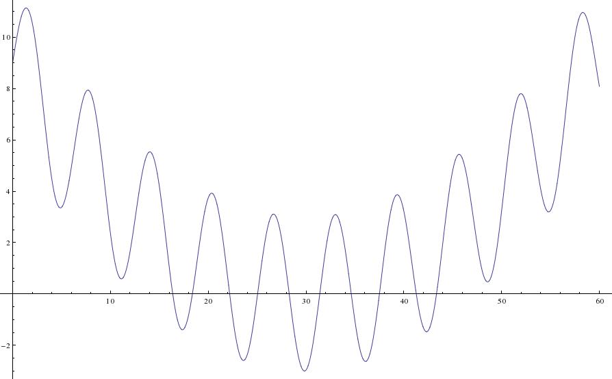
, for c a constant. There is a paper by Kofke(2002) that justifies this temperature set as it yields a constant acceptance ratio between cores under certain conditions. Indeed, the acceptance ratio (the fraction of metropolis moves that succeeded between cores) are roughly constant, as shown below:

    [1] 0.7227723
    [1] 0.7926793
    [1] 0.710171
    [1] 0.8037804
    [1] 0.7191719
    [1] 0.7974797
    [1] 0.729673
    [1] 0.8223822
    [1] 0.8184818
    [1] 0.8445845
    

    Earl D.J. & Deem M.W. (2005). Parallel tempering: Theory, applications, and new perspectives, Physical Chemistry Chemical Physics, 7 (23) 3910. DOI:
    Kofke D.A. (2002). On the acceptance probability of replica-exchange Monte Carlo trials, The Journal of Chemical Physics, 117 (15) 6911. DOI:

    Easy 3-Minute Guide to Making apply() Parallel over Distributed Grids and Clusters in R

    Last week I attended a workshop on how to run highly parallel distributed jobs on the Open Science Grid (osg). There I met Derek Weitzel who has made an excellent contribution to advancing R as a high performance computing language by developing BoscoR. BoscoR greatly facilitates the use of the already existing package “GridR” by allowing the R user to use Bosco to manage the submission of jobs. It seems no matter how many kinds of queue-submission system I become familiar with (torque,sge,condor), the current cluster I’m working on uses something foreign and so I have to relearn how to write a job submission file. One of the two major selling points of Bosco is that it allows the user to write one job submission file locally (based on HTCondor) and use it to submit jobs on various remote clusters all using different interfaces. The second major selling point is that Bosco will manage work sharing if you have access to more than one cluster, that is it will submit jobs to each cluster proportional to how unburdened that cluster is, which is great if you have access to 3 clusters. It means the users apply jobs will get through the queue as quickly as possible by cleverly distributing the work over all available clusters. Hopefully that will have convinced you that Bosco is worth having, now lets proceed with how to use it. I will illustrate the process by using Duke University’s cluster, the DSCR. There are three steps: 1) Installing Bosco 2) Installing GridR 3) Running a test job.

    Installing Bosco

    First go ahead and download Bosco, the sign-up is only for the developers to get an idea of how many people are using it. Detailed install instructions can be found here but I will also go through the steps.

    [lindon@laptop Downloads]$ tar xvzf ./bosco_quickstart.tar.gz
    [lindon@laptop Downloads]$ ./bosco_quickstart
    

    The executable will then ask some questions:

    Do you want to install Bosco? Select y/n and press [ENTER]: y
    Type the cluster name and press [ENTER]: dscr-login-01.oit.duke.edu
    When prompted “Type your name at dscr-login-01.oit.duke.edu (default YOUR_USER) and press [ENTER]: NetID
    When prompted “Type the queue manager for login01.osgconnect.net (pbs, condor, lsf, sge, slurm) and press [ENTER]: sge
    Then when prompted “NetID@dscr-login-01.oit.duke.edu’s password: XXXXXXX

    For duke users, the HostName of the DCSR is dscr-login-01.oit.duke.edu. You login with your NetID and the queue submission system is the Sun Grid Engine, so type sge. If you already have SSH-Keys set up then I think the last question gets skipped. That takes care of the installation. You can now try submitting on the remote cluster locally from your laptop. Download this test executable and this submission file. Start Bosco and try submitting a job.

    [msl33@hotel ~/tutorial-bosco]$ source ~/bosco/bosco_setenv
    [msl33@hotel ~/tutorial-bosco]$ bosco_start
    BOSCO Started
    [msl33@hotel ~/tutorial-bosco]$ condor_submit bosco01.sub 
    Submitting job(s).
    1 job(s) submitted to cluster 70.
    [msl33@hotel ~/tutorial-bosco]$ condor_q
    
    
    -- Submitter: hotel.stat.duke.edu : <127.0.0.1:11000?sock=21707_cbb6_3> : hotel.stat.duke.edu
     ID      OWNER            SUBMITTED     RUN_TIME ST PRI SIZE CMD               
      70.0   msl33           8/31 12:08   0+00:00:00 I  0   0.0  short.sh          
    
    1 jobs; 0 completed, 0 removed, 1 idle, 0 running, 0 held, 0 suspended
    

    This is the result if all has worked well. Note that you need to start Bosco by the above two lines.


    Installing GridR

    The current version of GridR on CRAN is an older version doesn’t support job submission by bosco. It will when CRAN gets the latest version of GridR but until then you need to install GridR from source so download it here and install it:

    install.packages("~/Downloads/GridR_0.9.7.tar.gz", repos=NULL, type="source")


    Running a Parallel Apply on the Cluster

    Consider a toy example which approximates pi by monte-carlo.

    montecarloPi <- function(trials, inst) {
      count = 0
      for(i in 1:trials) {
        if((runif(1,0,1)^2 + runif(1,0,1)^2)<1) {
          count = count + 1
        }
      }
      return((count*4)/trials)
    }
    

    One can now use grid.apply from the GridR package combined with Bosco to submit jobs on the remote cluster from within the users local R session.

    # load the GridR library
    library("GridR")
    grid.init(service="bosco.direct", localTmpDir="tmp")
    # Send 10 instances of the montecarloPi
    grid.apply("pi_estimate", montecarloPi, 10000000, c(1:10), batch=c(2))
    

    You can then see how your jobs are getting on by the “grid.printJobs()” command.
    parallel grid apply
    When it completes, “pi_estimate” will be a list object with 10 elements containing approximations to pi. Obviously, there is an overhead with submitting jobs and also a lag time while these jobs get through the queue. One must balance this overhead with the computational time required to complete a single iteration of the apply function. Bosco will create and submit a job for every iteration of the apply function. If each iteration does not take too long but there exists a great many of them to perform, one could consider blocking these operations into, say, 10 jobs so that the queue lag and submission overhead is negligible in comparison to the time taken to complete no_apply_iteraions/10 computations, which also saves creating a large number of jobs on the cluster which might aggravate other users. One can also add clusters to bosco using the “bosco_cluster –add” command, so that jobs are submitted to whichever cluster has the most free cores available. All in all this is a great aid for those doing computationally intensive tasks and makes parallel work-sharing very easy indeed.