This post is a review of the “GENERALIZED DOUBLE PARETO SHRINKAGE” Statistica Sinica (2012) paper by Armagan, Dunson and Lee.
Consider the regression model \(Y=X\beta+\varepsilon\) where we put a generalized double pareto distribution as the prior on the regression coefficients \(\beta\). The GDP distribution has density
$$\begin{equation}
f(\beta|\xi,\alpha)=\frac{1}{2\xi}\left( 1+\frac{|\beta|}{\alpha\xi} \right)^{-(\alpha+1)}.
\label{}
\end{equation}$$
GDP as Scale Mixture of Normals
The GDP distribution can be conveniently represented as a scale mixture of normals. Let
$$\begin{align*}
\beta_{i}|\phi,\tau_{i} &\sim N(0,\phi^{-1}\tau_{i})\\
\tau_{i}|\lambda_{i}&\sim Exp(\frac{\lambda_{i}^{2}}{2})\\
\lambda_{i}&\sim Ga(\alpha,\eta)\\
\end{align*}$$
then \(\beta|\phi \sim GDP(\xi=\frac{\eta}{\sqrt{\phi}\alpha},\alpha)\).
To see this first note that \(\beta_{i}|\phi,\lambda_{i}\) has a Laplace or Double Exponential distribution with rate parameter \(\sqrt{\phi}\lambda_{i}\).
$$\begin{align*}
p(\beta_{i}|\phi,\lambda_{i})&=\int p(\beta_{i}|\phi,\tau_{i})p(\tau_{i}|\lambda_{i})d\tau_{i}\\
\psi(t)&=\int e^{it\beta_{i}} \int p(\beta_{i}|\phi,\tau_{i})p(\tau_{i}|\lambda_{i})d\tau_{i} d\beta_{i}\\
&=\int \int e^{it\beta_{i}}p(\beta_{i}|\phi,\tau_{i})d\beta_{i}p(\tau_{i}|\lambda_{i})d\tau_{i}\\
&=\int e^{-\frac{1}{2}\frac{\tau_{i}}{\phi}t^{2}}p(\tau_{i}|\lambda_{i})d\tau_{i}\\
&=\frac{\lambda_{i}^{2}}{2} \int e^{-\frac{1}{2}(\frac{t^{2}}{\phi}+\frac{\lambda_{i}^{2}}{2})\tau_{i}}d\tau_{i}\\
&=\frac{\phi\lambda_{i}^{2}}{t^{2}+\phi\lambda_{i}^{2}},
\end{align*}$$
which is the characteristic function of a Double Exponential distribution with rate parameter \(\sqrt{\phi}\lambda_{i}\).
Lastly
$$\begin{align*}
p(\beta_{i}|\phi)&=\int p(\beta_{i}|\phi,\lambda_{i})p(\lambda_{i})d\lambda_{i}\\
&=\frac{1}{2}\sqrt{\phi}\frac{\eta^{\alpha}}{\Gamma(\alpha)}\frac{\Gamma(\alpha+1)}{(\eta+\sqrt{\phi}|\beta_{i}|)^{\alpha+1}}\\
&=\frac{1}{2}\frac{\sqrt{\phi}\alpha}{\eta}\left( 1+\frac{\sqrt{\phi}\alpha}{\eta}\frac{|\beta_{i}|}{\alpha} \right)^{-(\alpha+1)},
\end{align*}$$
which is the density of a \(GDP(\xi=\frac{\eta}{\sqrt{\phi}\alpha},\alpha)\).
EM Algorithm
\(\tau_{i}\) and \(\lambda_{i}\) are treated as missing data for each \(i\).
\begin{align*}
Q(\beta,\phi||\beta^{(t)},\phi^{(t)})&=c+\mathbb{E}_{\tau,\lambda}\left[ \log p(\beta,\phi|Y,\tau,\lambda)|\beta^{(t)},\phi^{(t)} \right]\\
&=\frac{n+p-3}{2}\log\phi – \frac{\phi}{2}||Y-X\beta||^{2}-\frac{\phi}{2}\sum_{i=1}^{p}\beta_{i}^{2}\mathbb{E}\left[ \frac{1}{\tau_{i}} \right]\\
\end{align*}
Expectation
For the iterated expectation one needs the distribution \(\tau_{i}|\lambda_{i},\beta_{i},\phi\) and \(\lambda_{i}|\beta_{i},\phi\).
\begin{align*}
p(\tau_{i}|\beta_{i},\lambda_{i},\phi)&\propto p(\beta_{i}|\phi,\tau_{i})p(\tau_{i}|\lambda_{i})\\
&\propto \left( \frac{1}{\tau_{i}} \right)^{\frac{1}{2}}e^{-\frac{1}{2}(\frac{\phi \beta_{i}^{2}}{\tau_{i}}+\lambda_{i}^{2}\tau_{i})}
\end{align*}
This is the kernel of a Generalized Inverse Gaussian distribution, specifically \(p(\tau_{i}|\beta_{i},\lambda_{i},\phi)=GIG(\tau_{i}:\lambda_{i}^{2},\phi \beta_{i}^{2},\frac{1}{2})\).
By a standard change of variables it follows that \(p(\frac{1}{\tau_{i}}|\beta_{i},\lambda_{i},\phi)=IG(\frac{1}{\tau_{i}}:\sqrt{\frac{\lambda_{i}^{2}}{\phi \beta_{i}^{2}}},\lambda_{i}^{2})\) and so \(\mathbb{E}\left[ \frac{1}{\tau_{i}}|\lambda_{i},\beta^{(t)},\phi^{(t)} \right]=\frac{\lambda_{i}}{\sqrt{\phi^{(t)}}|\beta_{i}^{(t)}|}\).
Recall that \(p(\beta_{i}|\phi,\lambda_{i})\) has a double exponential distribution with rate \(\sqrt{\phi}\lambda_{i}\).
Hence from \(p(\lambda_{i}|\beta_{i},\phi)\propto p(\beta_{i}|\lambda_{i},\phi)p(\lambda_{i})\) it follows that \(\lambda_{i}|\beta_{i},\phi \sim Ga(\alpha+1,\eta+\sqrt{\phi}|\beta_{i}|)\), then performing the expectation with respect to \(\lambda_{i}\) yields
\begin{align*}
\mathbb{E}\left[ \frac{1}{\tau_{i}}|\beta^{(t)},\phi^{(t)} \right]=\left( \frac{\alpha+1}{\eta+\sqrt{\phi^{t}}|\beta_{i}^{(t)}|} \right)\left( \frac{1}{\sqrt{\phi^{(t)}}|\beta_{i}^{(t)}|} \right)
\end{align*}
Maximization
Writing \(D^{(t)}=diag(\mathbb{E}[\frac{1}{\tau_{1}}],\dots,\mathbb{E}[\frac{1}{\tau_{p}}])\) the function to maximize is
\begin{align*}
Q(\beta,\phi||\beta^{(t)},\phi^{(t)})&=c+\mathbb{E}_{\tau,\lambda}\left[ \log p(\beta,\phi|Y,\tau,\lambda)|\beta^{(t)},\phi^{(t)} \right]\\
&=\frac{n+p-3}{2}\log\phi – \frac{\phi}{2}||Y-X\beta||^{2}-\frac{\phi}{2}\beta^{‘}D^{(t)}\beta,\\
\end{align*}
which is maximized by letting
\begin{align*}
\beta^{(t+1)}&=(X^{‘}X+D^{(t)})^{-1}X^{‘}Y\\
\phi^{(t+1)}&=\frac{n+p-3}{Y^{‘}(I-X(X^{‘}X+D^{(t)})^{-1}X^{‘})Y}\\
&=\frac{n+p-3}{||Y-X\beta^{(t+1)}||^{2}+\beta^{(t+1)’}D^(t)\beta^{(t+1)}}\\
\end{align*}
R CPP Code
#include <RcppArmadillo.h>
// [[Rcpp::depends(RcppArmadillo)]]

using namespace Rcpp;
using namespace arma;

double gdp_log_posterior_density(int no, int p, double alpha, double eta, const Col<double>& yo, const Mat<double>& xo, const Col<double>& B,double phi);

// [[Rcpp::export]]
List gdp_em(NumericVector ryo, NumericMatrix rxo, SEXP ralpha, SEXP reta){

	//Define Variables//
	int p=rxo.ncol();
	int no=rxo.nrow();
	double eta=Rcpp::as<double >(reta);
	double alpha=Rcpp::as<double >(ralpha);

	//Create Data//
	arma::mat xo(rxo.begin(), no, p, false);
	arma::colvec yo(ryo.begin(), ryo.size(), false);
	yo-=mean(yo);

	//Pre-Processing//
	Col<double> xoyo=xo.t()*yo;
	Col<double> B=xoyo/no;
	Col<double> Babs=abs(B);
	Mat<double> xoxo=xo.t()*xo;
	Mat<double> D=eye(p,p);
	Mat<double> Ip=eye(p,p);
	double yoyo=dot(yo,yo);
	double deltaB;
	double deltaphi;
	double phi=no/dot(yo-xo*B,yo-xo*B);
	double lp;

	//Create Trace Matrices
	Mat<double> B_trace(p,20000);
	Col<double> phi_trace(20000);
	Col<double> lpd_trace(20000);

	//Run EM Algorithm//
	cout << "Beginning EM Algorithm" << endl;
	int t=0;
	B_trace.col(t)=B;
	phi_trace(t)=phi;
	lpd_trace(t)=gdp_log_posterior_density(no,p,alpha,eta,yo,xo,B,phi);
	do{
		t=t+1;


		Babs=abs(B);
		D=diagmat(sqrt(((eta+sqrt(phi)*Babs)%(sqrt(phi)*Babs))/(alpha+1)));
		B=D*solve(D*xoxo*D+Ip,D*xoyo);

		phi=(no+p-3)/(yoyo-dot(xoyo,B));

		//Store Values//
		B_trace.col(t)=B;
		phi_trace(t)=phi;
		lpd_trace(t)=gdp_log_posterior_density(no,p,alpha,eta,yo,xo,B,phi);

		deltaB=dot(B_trace.col(t)-B_trace.col(t-1),B_trace.col(t)-B_trace.col(t-1));
		deltaphi=phi_trace(t)-phi_trace(t-1);
	} while((deltaB>0.00001 || deltaphi>0.00001) && t<19999);
	cout << "EM Algorithm Converged in " << t << " Iterations" << endl;

	//Resize Trace Matrices//
	B_trace.resize(p,t);
	phi_trace.resize(t);
	lpd_trace.resize(t);

	return Rcpp::List::create(
			Rcpp::Named("B") = B,
			Rcpp::Named("B_trace") = B_trace,
			Rcpp::Named("phi") = phi,
			Rcpp::Named("phi_trace") = phi_trace,
			Rcpp::Named("lpd_trace") = lpd_trace
			) ;

}


double gdp_log_posterior_density(int no, int p, double alpha, double eta, const Col<double>& yo, const Mat<double>& xo, const Col<double>& B,double phi){

	double lpd;
	double xi=eta/(sqrt(phi)*alpha);
	lpd=(double)0.5*((double)no-1)*log(phi/(2*M_PI))-p*log(2*xi)-(alpha+1)*sum(log(1+abs(B)/(alpha*xi)))-0.5*phi*dot(yo-xo*B,yo-xo*B)-log(phi);
	return(lpd);

}
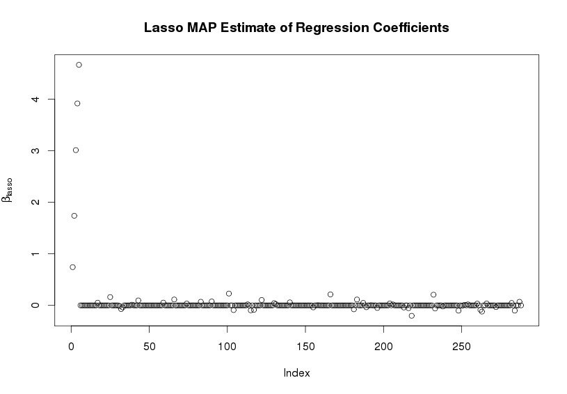
An Example in R
rm(list=ls())
library(Rcpp)
library(RcppArmadillo)
sourceCpp("src/gdp_em.cpp")

#Generate Design Matrix
set.seed(3)
no=100
foo=rnorm(no,0,1)
sd=4
xo=cbind(foo+rnorm(no,0,sd),foo+rnorm(no,0,sd),foo+rnorm(no,0,sd),foo+rnorm(no,0,sd),foo+rnorm(no,0,sd),foo+rnorm(no,0,sd),foo+rnorm(no,0,sd),foo+rnorm(no,0,sd))
for(i in 1:40) xo=cbind(xo,foo+rnorm(no,0,sd),foo+rnorm(no,0,sd),foo+rnorm(no,0,sd),foo+rnorm(no,0,sd),foo+rnorm(no,0,sd),foo+rnorm(no,0,sd),foo+rnorm(no,0,sd))

#Scale and Center Design Matrix
xo=scale(xo,center=T,scale=F)
var=apply(xo^2,2,sum)
xo=scale(xo,center=F,scale=sqrt(var/no))

#Generate Data under True Model
p=dim(xo)[2]
b=rep(0,p)
b[1]=1
b[2]=2
b[3]=3
b[4]=4
b[5]=5
xo%*%b
yo=xo%*%b+rnorm(no,0,1)
yo=yo-mean(yo)

#Run GDP
gdp=gdp_em(yo,xo,100,100)

#Posterior Density Increasing at Every Iteration?
gdp$lpd_trace[2:dim(gdp$lpd_trace)[1],1]-gdp$lpd_trace[1:(dim(gdp$lpd_trace)[1]-1),1]>=0
mean(gdp$lpd_trace[2:dim(gdp$lpd_trace)[1],1]-gdp$lpd_trace[1:(dim(gdp$lpd_trace)[1]-1),1]>=0)

#Plot Results
plot(gdp$B,ylab=expression(beta[GDP]),main="GDP MAP Estimate of Regression Coefficients")

WEST M. (1987). On scale mixtures of normal distributions, Biometrika, 74 (3) 646-648. DOI: http://dx.doi.org/10.1093/biomet/74.3.646
Artin Armagan, David Dunson, & Jaeyong Lee (2011). Generalized double Pareto shrinkage Statistica Sinica 23 (2013), 119-143 arXiv: 1104.0861v4
Figueiredo M.A.T. (2003). Adaptive sparseness for supervised learning, IEEE Transactions on Pattern Analysis and Machine Intelligence, 25 (9) 1150-1159. DOI: http://dx.doi.org/10.1109/tpami.2003.1227989
Also see this similar post on the Bayesian lasso.

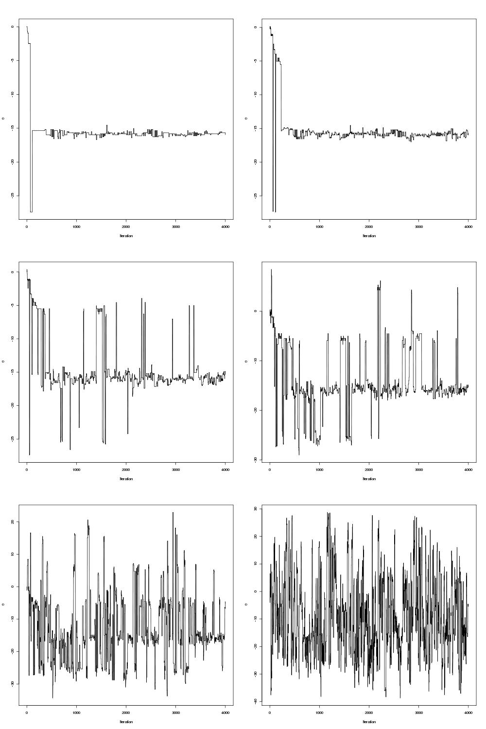
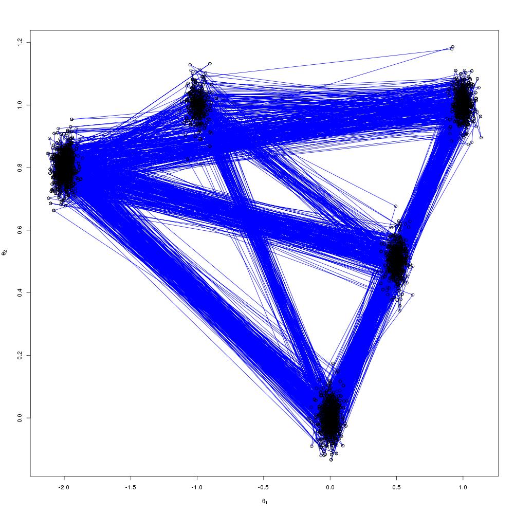
 , algorithm on it to try and improve the mixing but the problem was that it was written in R and I’m used to writing parallel code in C/C++ with OpenMP or MPI. Previously I wrote about a parallel tempering algorithm with an implementation in C++ using OpenMP and so I thought I would try and code up the same sort of thing in R as a warm-up exercise before I started with the full
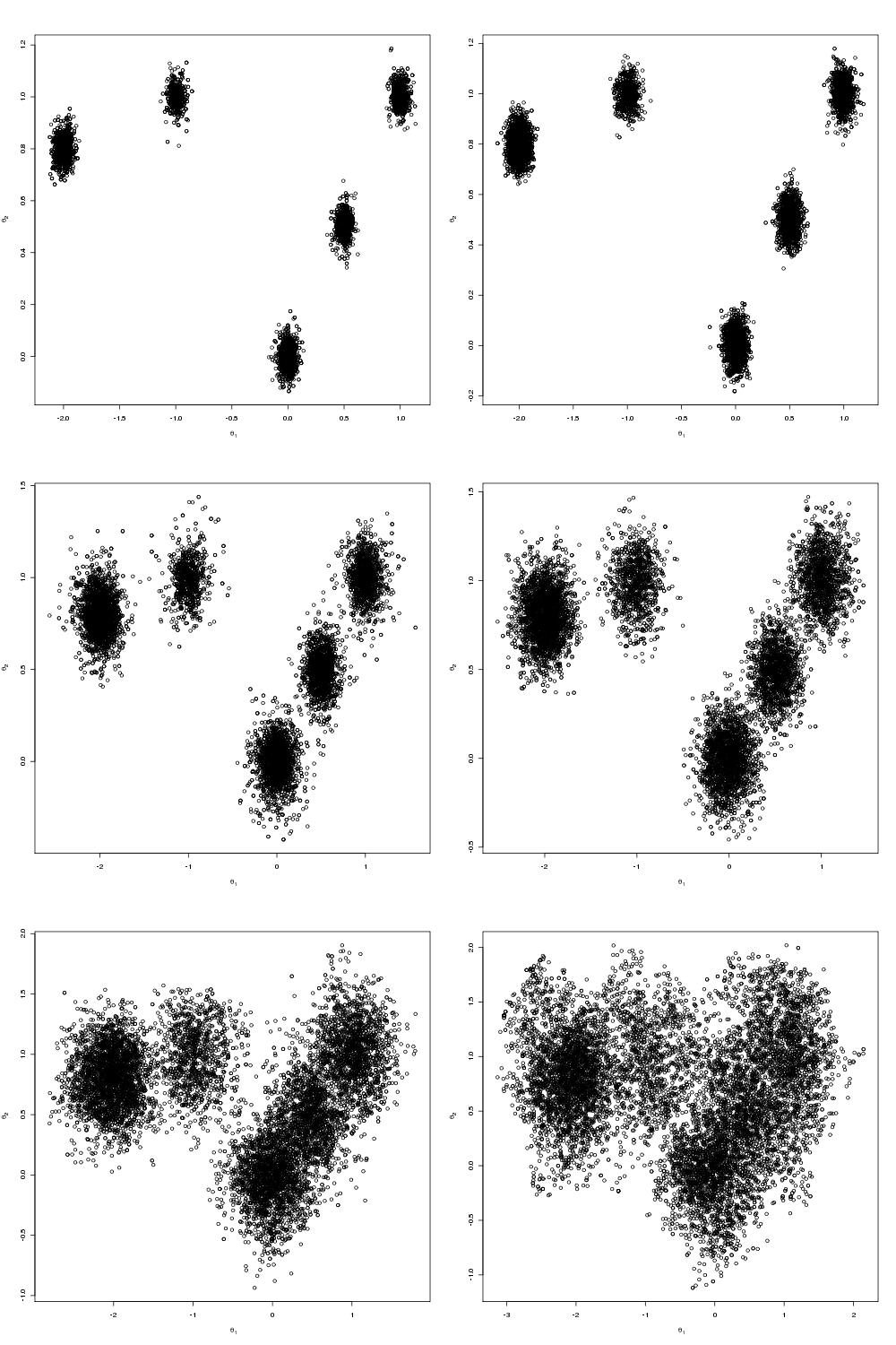
 , for c a constant. There is a paper by Kofke(2002) that justifies this temperature set as it yields a constant acceptance ratio between cores under certain conditions. Indeed, the acceptance ratio (the fraction of metropolis moves that succeeded between cores) are roughly constant, as shown below:
 is independent of
  given
given 
 \ \ \ \ \ (1)")
 \ \ \ \ \ (2)")
 \propto \frac{1}{\lambda^{2}} \ \ \ \ \ (3)")
 \ \ \ \ \ (4)")
 \ \ \ \ \ (5)")
 and
and  \ \ \ \ \ (6)")
 \ \ \ \ \ (7)")
 \propto 1 \ \ \ \ \ (8)")
 \ \ \ \ \ (9)")
 \ \ \ \ \ (10)")