Metropolis Adjusted Langevin Algorithm (MALA)
Haven’t dumped much code here in a while. Here’s a Julia implementation of MALA with an arbitrary preconditioning matrix M. Potentially I might use this in the future.
Generic Julia Implementation
Arguments are a function to evaluate the logdensity, function to evaluate the gradient, a step size h, a preconditioning matrix M, number of iterations and an initial parameter value.
function mala(logdensity,gradient,h,M,niter,θinit)
        function gradientStep(θ,t)
                θ-t*M*gradient(θ)
        end
        θtrace=Array{Float64}(length(θinit),niter)
        θ=θinit
        θtrace[:,1]=θinit
        for i=2:niter
                θold=θ
                θ=rand(MvNormal(gradientStep(θ,0.5*h),h*M))
                d=logdensity(θ) - logdensity(θold) + logpdf(MvNormal(gradientStep(θ,0.5*h),h*M),θold) - logpdf(MvNormal(gradientStep(θold,0.5*h),h*M),θ)
                if(!(log(rand(Uniform(0,1)))<d))
                        θ=θold
                end
                θtrace[:,i]=θ
        end
        θtrace
end
Don’t forget to use the Distributions package of Julia.
Bivariate Normal Example
Consider a Bivariate Normal as an example
ρ²=0.8
Σ=[1 ρ²;ρ² 1]

function logdensity(θ)
        logpdf(MvNormal(Σ),θ)
end

function gradient(θ)
        Σ\θ
end
and now the code to generate the plots and results
niter=1000
h=1/eigs(inv(Σ),nev=1)[1][1]
@time draws=mala(logdensity,gradient,h,eye(2),niter,[5,50]);
sum(map(t -> draws[:,t]!=draws[:,t-1],2:niter))/(niter-1)
@time pdraws=mala(logdensity,gradient,h,Σ,niter,[5,50]);
sum(map(t -> pdraws[:,t]!=pdraws[:,t-1],2:niter))/(niter-1)
function logdensity2d(x,y)
logdensity([x,y])
end
x = -30:0.1:30
y = -30:0.1:50
X = repmat(x',length(y),1)
Y = repmat(y,1,length(x))
Z = map(logdensity2d,Y,X)
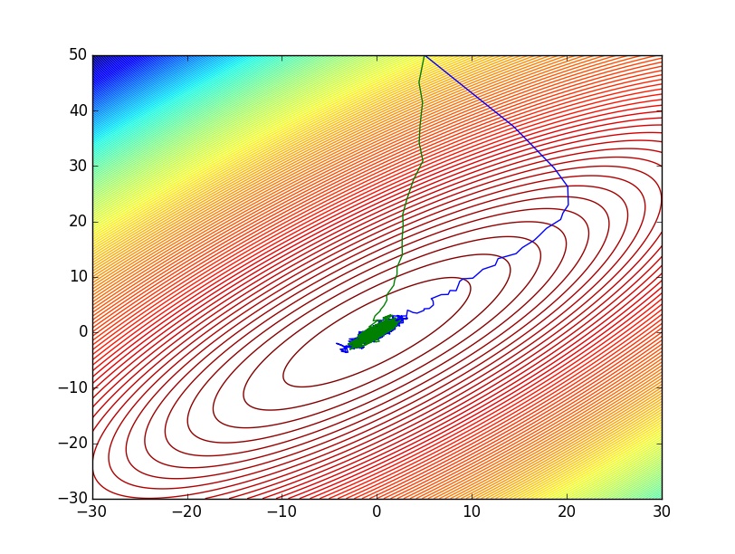
p1 = contour(x,y,Z,200)
plot(vec(draws[1,:]),vec(draws[2,:]))
plot(vec(pdraws[1,:]),vec(pdraws[2,:]))
pdraws uses the covariance matrix Σ as the preconditioning matrix, whereas the first uses an identity matrix, resulting in the original MALA algorithm. The traceplot of draws from MALA and preconditioned MALA are shown in blue and green respectively…
Traceplots for MALA and preconditioned MALA
Effective Sample Sizes in R
We can use the julia “RCall” package to switch over to R and use the coda library to evaluate the minimum effective sample size for both of these MCMC algorithms.
julia> library(coda)

R> library(coda)

R> min(effectiveSize($(draws')))
[1] 22.02418

R> min(effectiveSize($(pdraws')))
[1] 50.85163
I didn’t tune the step size h in this example at all (you should).