Ages 10-12 Toy Exoplanet Detection

A major objection with the previous simulated light curves is that the baseline is rarely constnat. Instead, from what I have learned, it is a horrible mess of discontinuities and curves due to the telescope rotating and instruments heating up. I spoke to someone who said that there is some periodicity in the curve. It is easy to adapt the previous code to generalize it for a periodic background flux. Consider the model:
$f_{t} \sim N(b_{1} + a\text{sin}(\omega t)- b_{2}1_{ \left[ \tau_{1},\tau_{2} \right] }(t), \sigma^{2})$
which has two additional parameters, the amplitude a and the angular frequency omega, upon which I put priors:
$a \sim unif(0,b_{1})\\ \omega \sim unif(0,1)\\$
I’m not sure if the last one is justified, I’d need to talk to an exoplanet expert, but hopefully the background frequency is a lot less than the frequency at which measurements are being made.
The JAGS code looks like this:

model
{
for(t in 1 : N)
{
D[t] ~ dnorm(mu[t],s2)
mu[t] <- b[1]+ amp*sin(omega*t) - step(t - tau1)*step(tau2-t)*step(tau2-tau1) * b[2]
}
b[1] ~ dnorm(0.0,1.0E-6)T(0,)
b[2] ~ dnorm(0.0,1.0E-6)T(0,b[1])
tau1 ~ dunif(1,N)
tau2 ~ dunif(tau1,N)
s2 ~ dunif(0,100)
amp ~ dunif(0,b[1])
omega ~ dunif(0,1)
}

The code to call JAGS from R and make plots can be found here.

rm(list=ls())
library('rjags')

s2=5
bn=1000
dn=400
amp=1
omega=0.005
base=rnorm(bn,100,sqrt(s2))
drop=rnorm(dn,97,sqrt(s2))
t=seq(1,length(c(base,drop,base,base)),1)
sin=amp*sin(omega*t)
trace=c(base,drop,base,base)
trace=trace+sin

plot(trace,type="l",col="red",xlab="Time t",ylab="Flux")

datalist=list(
  D=trace,
  N=length(trace)
  )

jags <- jags.model(file.path('/home/grad/msl33/Dropbox/samsi/cp.bugs'),data = datalist, n.chains = 1, n.adapt = 500)
mcmc.samples=coda.samples(jags,c('b','tau1','tau2','amp','omega'),2000)
plot(mcmc.samples)

and I generated some fake data that looks like this:

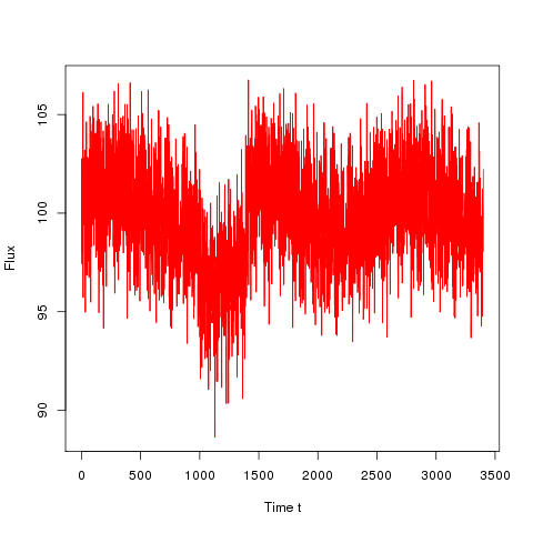
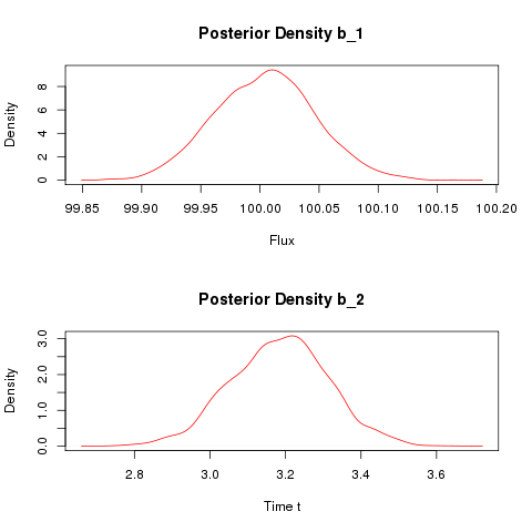
based on the parameters:
$b_{1}=100\\ b_{2}=3\\ a=1\\ \tau_{1}=1000\\ \tau_{2}=1400\\$