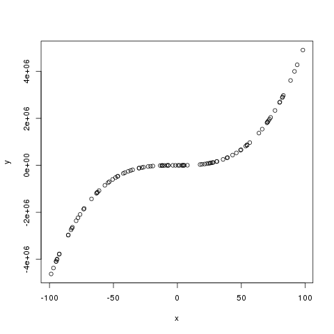
This post is just a brief example of how linear model theory can be used to perform polynomial regression. Consider getting some bivariate data that looks like this (downloadable here)

and suppose we wish to fit a 3rd degree polynomial to this data. We can write it as a linear model
which is a linear model because it is linear in the regression coefficients. The ordinary least squares estimator of the regression coefficients is then
This is implemented in the below R code
plot(x,y)
n=length(y)
int=rep(1,n)
X=cbind(x,x^2,x^3,int)
B=solve(t(X)%*%X)%*%t(X)%*%y
u=seq(-100,100,1)
v=B[4]+B[1]*u+B[2]*u^2+B[3]*u^3
lines(u,v,col="red")
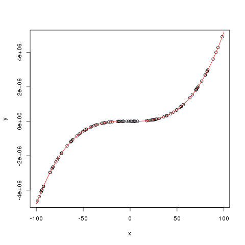
The array B contains the OLS estimates of the regression coefficients. The fitted polynomial is fitted below in red:

The extension to higher degree polynomials is simple, just add columns to the design matrix X.