Parallel Tempering in R with Rmpi

My office computer recently got a really nice upgrade and now I have 8 cores on my desktop to play with. I also at the same time received some code for a Gibbs sampler written in R from my adviser. I wanted to try a metropolis-coupled markov chain monte carlo, MC^{3}, algorithm on it to try and improve the mixing but the problem was that it was written in R and I’m used to writing parallel code in C/C++ with OpenMP or MPI. Previously I wrote about a parallel tempering algorithm with an implementation in C++ using OpenMP and so I thought I would try and code up the same sort of thing in R as a warm-up exercise before I started with the full MC^{3} algorithm. Sadly I don’t think there is any facility in R for OpenMP style parallelism. There are packages such as snow and multicore but these are very high level packages and don’t really allow one to control the finer details. There is, however, Rmpi. It is a little bit different from regular C/Fortran MPI implementations and I once had a very bad experience getting some Rmpi code to work for a project deadline, it wasn’t pretty, so I was a little reluctant to reconsider this package but if you look at the changelogs it is still being actively maintained and in the end I’m very happy with the outcome of this experiment. I tried to write the below code as generally as possible, so that it is easily adapted by myself, or others, in the future.

Target Density

First one needs to write a density one wishes to sample from

logdensity<-function(theta){
  #Distribution one wishes to sample from here.
  #It may be more convinient to pass a theta as a list
  sigma2=0.001;
  Sigma=matrix(0,2,2);
  Sigma[1,1]=sigma2;
  Sigma[2,2]=sigma2;
  density=dmvnorm(theta,c(0,0),Sigma)+dmvnorm(theta,c(-2,0.8),Sigma)+dmvnorm(theta,c(-1,1),Sigma)+dmvnorm(theta,c(1,1),Sigma)+dmvnorm(theta,c(0.5,0.5),Sigma);
  return(log(density))
}

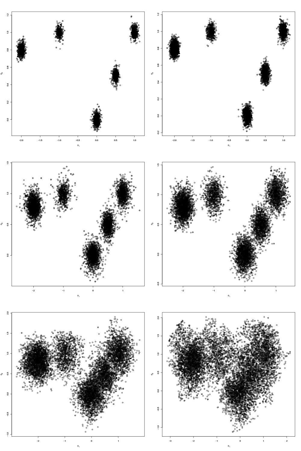
The density I chose was a mixture of 5 well-separated bi-variate Normals. One should note that it is probably cleanest to pass all the arguments to this function as a list theta. It wasn’t really necessary in this case but if you have a posterior distribution with a number of parameters of varying dimension then it would be much nicer as a list. In a future blog post I may change the target density to be the energy distribution of a Lennard-Jones cluster.

Parallel Tempering Algorithm

This too is written as a function because Rmpi allows you to pass the function to all slaves and execute it. It was basically the easiest way of writing it for Rmpi.

temper<-function(niter,Bmin,swap.interval){
  rank=mpi.comm.rank();
  size=mpi.comm.size();
  swap=0;
  swaps.attempted=0;
  swaps.accepted=0;
  
  #Higher ranks run the higher "temperatures" (~smaller fractional powers)
  B=rep(0,size-1);
  for(r in 1:size-1){
    temp=(r-1)/(size-2);
    B[r]=Bmin^temp;
  }
  
  
  #Create a list for proposal moves
  prop=rep(0,2);
  theta=matrix(0,niter,2)
  
  for(t in 2:niter){
    
    for(c in 1:length(prop))   prop=theta[t-1,c]+rnorm(1,0,0.1);
    
    #Calculate Log-Density at proposed and current position
    logdensity.current=logdensity(theta[t-1,])
    logdensity.prop=logdensity(prop);
    
    #Calculate log acceptance probability
    lalpha=B[rank]*(logdensity.prop-logdensity.current)
    
    if(log(runif(1))<lalpha){
      #Accept proposed move
      theta[t,]=prop;
      logdensity.current=logdensity.prop;
    }else{
      #Otherwise do not move
      theta[t,]=theta[t-1,];
    } 
    
    if(t%%swap.interval ==0){
      for(evenodd in 0:1){
        swap=0;
        logdensity.partner=0;
        if(rank%%2 == evenodd%%2){
          rank.partner=rank + 1;
          #ranks range from 1:size-1. Cannot have a partner rank == size
          if(0<rank.partner && rank.partner<size){
            #On first iteration, evens receive from above odd
            #On second iteration, odds receive from above evens
            logdensity.partner<-mpi.recv.Robj(rank.partner,rank.partner);
            lalpha = (B[rank]-B[rank.partner])*(logdensity.partner-logdensity.current);
            swaps.attempted=swaps.attempted+1;
            if(log(runif(1))<lalpha){
              swap=1;
              swaps.accepted=swaps.accepted+1;
            }
            mpi.send.Robj(swap,dest=rank.partner,tag=rank)
          }
          if(swap==1){
            thetaswap=theta[t,];
            mpi.send.Robj(thetaswap,dest=rank.partner,tag=rank)
            theta[t,]=mpi.recv.Robj(rank.partner,rank.partner)
          }
        }else{
          rank.partner=rank-1;
          #ranks range from 1:size-1. Cannot have a partner rank ==0
          if(0<rank.partner && rank.partner<size){
            #On first iteration, odds send to evens below
            #On second iteration, evens sent to odds below
            mpi.send.Robj(logdensity.current,dest=rank.partner,tag=rank);
            swap=mpi.recv.Robj(rank.partner,rank.partner);
          }
          if(swap==1){
            thetaswap=theta[t,];
            theta[t,]=mpi.recv.Robj(rank.partner,rank.partner);
            mpi.send.Robj(thetaswap,dest=rank.partner,tag=rank);
          }
        }
      }
    }
  }
  return(theta)
}

The bulk of the above code is the communication of each processor with its next nearest neighbors. Metropolis moves will be attempted every swap.interval iterations, an argument one can pass to the function. When this code block is entered, even rank processors will partner with their higher ranked odd neighbours (they have a high rank so higher temperature i.e. smaller fractional power – a more “melted down” target density). The higher odd partners will send their lower even partners the value of their density and then the lower even partners will calculate an acceptance probabilty. If the move succeeds the lower rank even processors send their higher rank odd processors a binary swap=1 telling the higher rank odd processors that a send/receive procedure will occur. The lower even rank sends the higher odd rank its parameters and then subsequently the higher odd rank sends its lower even rank its parameters. In this way a metropolis move between processors is achieved. Next, odd rank processors form partners with their higher even ranked neighbours (because we need to swap with processor rank 1, the target density). The same procedure occurs as before but swapping odd for even. More visually, first swaps are attempted between 2-3, 4-5, 6-7 etc and then swaps are attempted between 1-2, 3-4, 5-6. This is almost like a merge-sort style algorithm. One can see how the parameters could be passed from 3 down to 2 and then from 2 down to 1. The main point is that each processor attempts a swap with its nearest-neighbours, the one above and the one below, every swap.interval iterations.
With these functions defined one can now proceed to set up the mpi communicator/world.

Rmpi

First spawn some slaves.

library(Rmpi)
mpi.spawn.Rslaves(nslaves=6)

If it worked, you should see something like this:

> mpi.spawn.Rslaves(nslaves=6)
	6 slaves are spawned successfully. 0 failed.
master (rank 0, comm 1) of size 7 is running on: cabbage 
slave1 (rank 1, comm 1) of size 7 is running on: cabbage 
slave2 (rank 2, comm 1) of size 7 is running on: cabbage 
slave3 (rank 3, comm 1) of size 7 is running on: cabbage 
slave4 (rank 4, comm 1) of size 7 is running on: cabbage 
slave5 (rank 5, comm 1) of size 7 is running on: cabbage 
slave6 (rank 6, comm 1) of size 7 is running on: cabbage 

(yes, my office computer was named cabbage, lettuce is the one next to me). One can then send the function definitions to the slave processors.

niter=3000
Bmin=0.005
swap.interval=3
#Send to slaves some required data
mpi.bcast.Robj2slave(niter)
mpi.bcast.Robj2slave(Bmin)
mpi.bcast.Robj2slave(swap.interval)
#Send to slaves the logdensity function
mpi.bcast.Robj2slave(logdensity)
#Send to slaves the temper function
mpi.bcast.Robj2slave(temper) 
#Send to slaves the dmvnorm function
mpi.bcast.Robj2slave(dmvnorm) 

If you want to make sure that the slaves have the correct function definition, one can execute the command mpi.remote.exec(temper) and this will return the function definition. That is all, now it can be run.

mcmc=mpi.remote.exec(temper(niter,Bmin,swap.interval))

This returns a list object containing the mcmc draws for each slave.
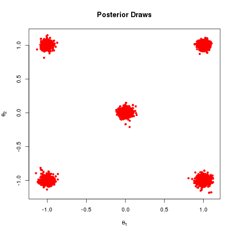
Results

The end product is something that looks like this
parallel tempering mixing
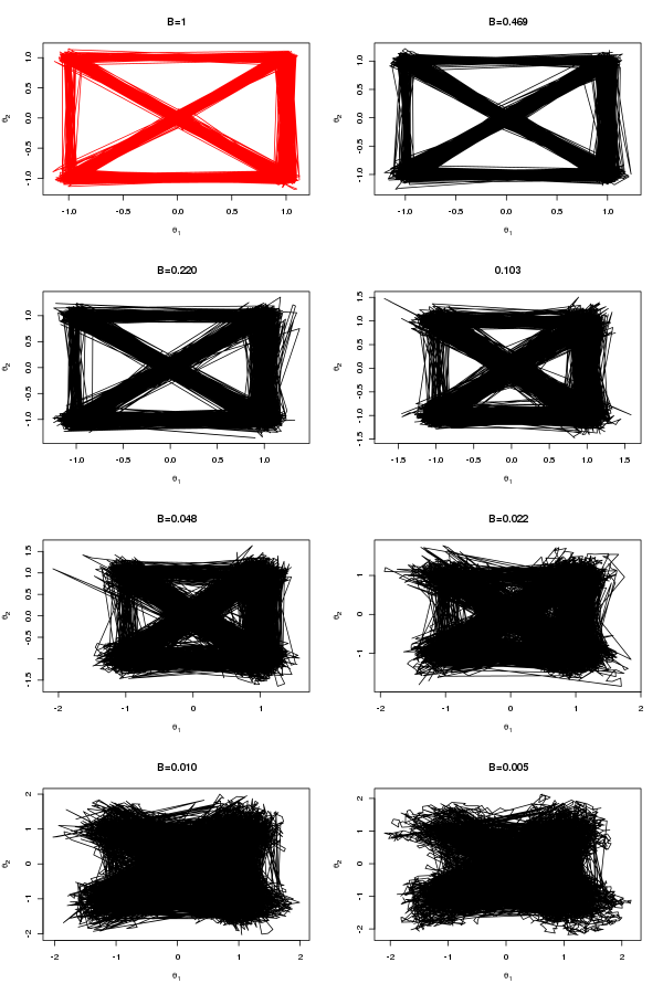
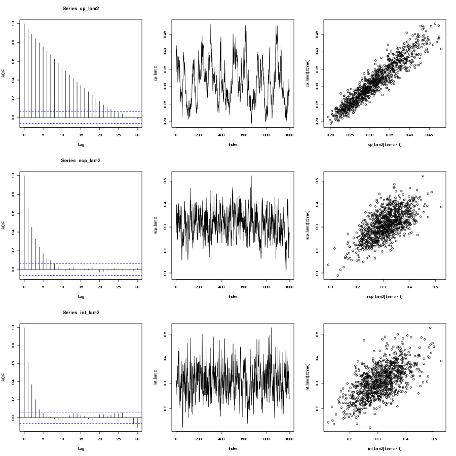
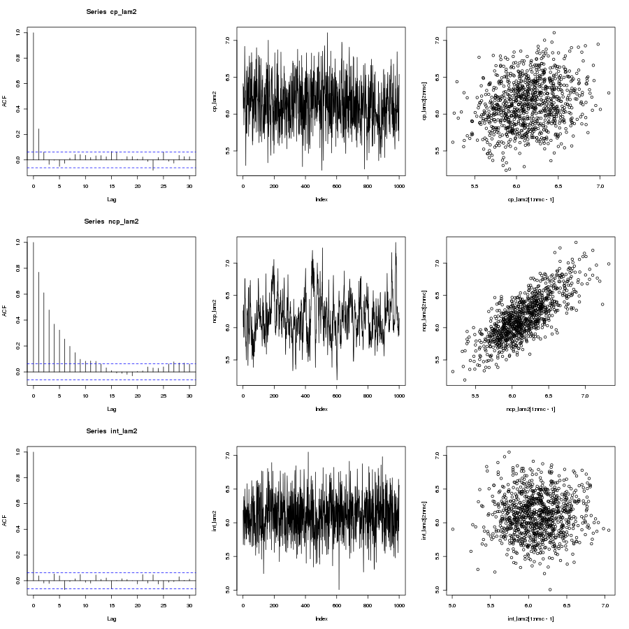
Which are the draws (in black) from the target distribution. It is also useful to build up intuition for parallel tempering to look at what is happening on the other processors. The draws for all processors are shown below:
parallel tempering draws for each processor

N.B. Although my computer only has 8 cores I tried running the code 12 slaves. At first I was concerned that the MPI communications would enter a deadlock and the code would hang but it didn’t, so it seems you can scale up the number of slaves above the number of cores.

Temperature Set

Notice that the temperature set used in the code has the property that \frac{\beta_{n}}{\beta_{n+1}}=c, for c a constant. There is a paper by Kofke(2002) that justifies this temperature set as it yields a constant acceptance ratio between cores under certain conditions. Indeed, the acceptance ratio (the fraction of metropolis moves that succeeded between cores) are roughly constant, as shown below:

[1] 0.7227723
[1] 0.7926793
[1] 0.710171
[1] 0.8037804
[1] 0.7191719
[1] 0.7974797
[1] 0.729673
[1] 0.8223822
[1] 0.8184818
[1] 0.8445845

Earl D.J. & Deem M.W. (2005). Parallel tempering: Theory, applications, and new perspectives, Physical Chemistry Chemical Physics, 7 (23) 3910. DOI:
Kofke D.A. (2002). On the acceptance probability of replica-exchange Monte Carlo trials, The Journal of Chemical Physics, 117 (15) 6911. DOI:

Easy 3-Minute Guide to Making apply() Parallel over Distributed Grids and Clusters in R

Last week I attended a workshop on how to run highly parallel distributed jobs on the Open Science Grid (osg). There I met Derek Weitzel who has made an excellent contribution to advancing R as a high performance computing language by developing BoscoR. BoscoR greatly facilitates the use of the already existing package “GridR” by allowing the R user to use Bosco to manage the submission of jobs. It seems no matter how many kinds of queue-submission system I become familiar with (torque,sge,condor), the current cluster I’m working on uses something foreign and so I have to relearn how to write a job submission file. One of the two major selling points of Bosco is that it allows the user to write one job submission file locally (based on HTCondor) and use it to submit jobs on various remote clusters all using different interfaces. The second major selling point is that Bosco will manage work sharing if you have access to more than one cluster, that is it will submit jobs to each cluster proportional to how unburdened that cluster is, which is great if you have access to 3 clusters. It means the users apply jobs will get through the queue as quickly as possible by cleverly distributing the work over all available clusters. Hopefully that will have convinced you that Bosco is worth having, now lets proceed with how to use it. I will illustrate the process by using Duke University’s cluster, the DSCR. There are three steps: 1) Installing Bosco 2) Installing GridR 3) Running a test job.

Installing Bosco

First go ahead and download Bosco, the sign-up is only for the developers to get an idea of how many people are using it. Detailed install instructions can be found here but I will also go through the steps.

[lindon@laptop Downloads]$ tar xvzf ./bosco_quickstart.tar.gz
[lindon@laptop Downloads]$ ./bosco_quickstart

The executable will then ask some questions:

Do you want to install Bosco? Select y/n and press [ENTER]: y
Type the cluster name and press [ENTER]: dscr-login-01.oit.duke.edu
When prompted “Type your name at dscr-login-01.oit.duke.edu (default YOUR_USER) and press [ENTER]: NetID
When prompted “Type the queue manager for login01.osgconnect.net (pbs, condor, lsf, sge, slurm) and press [ENTER]: sge
Then when prompted “NetID@dscr-login-01.oit.duke.edu’s password: XXXXXXX

For duke users, the HostName of the DCSR is dscr-login-01.oit.duke.edu. You login with your NetID and the queue submission system is the Sun Grid Engine, so type sge. If you already have SSH-Keys set up then I think the last question gets skipped. That takes care of the installation. You can now try submitting on the remote cluster locally from your laptop. Download this test executable and this submission file. Start Bosco and try submitting a job.

[msl33@hotel ~/tutorial-bosco]$ source ~/bosco/bosco_setenv
[msl33@hotel ~/tutorial-bosco]$ bosco_start
BOSCO Started
[msl33@hotel ~/tutorial-bosco]$ condor_submit bosco01.sub 
Submitting job(s).
1 job(s) submitted to cluster 70.
[msl33@hotel ~/tutorial-bosco]$ condor_q


-- Submitter: hotel.stat.duke.edu : <127.0.0.1:11000?sock=21707_cbb6_3> : hotel.stat.duke.edu
 ID      OWNER            SUBMITTED     RUN_TIME ST PRI SIZE CMD               
  70.0   msl33           8/31 12:08   0+00:00:00 I  0   0.0  short.sh          

1 jobs; 0 completed, 0 removed, 1 idle, 0 running, 0 held, 0 suspended

This is the result if all has worked well. Note that you need to start Bosco by the above two lines.


Installing GridR

The current version of GridR on CRAN is an older version doesn’t support job submission by bosco. It will when CRAN gets the latest version of GridR but until then you need to install GridR from source so download it here and install it:

install.packages("~/Downloads/GridR_0.9.7.tar.gz", repos=NULL, type="source")


Running a Parallel Apply on the Cluster

Consider a toy example which approximates pi by monte-carlo.

montecarloPi <- function(trials, inst) {
  count = 0
  for(i in 1:trials) {
    if((runif(1,0,1)^2 + runif(1,0,1)^2)<1) {
      count = count + 1
    }
  }
  return((count*4)/trials)
}

One can now use grid.apply from the GridR package combined with Bosco to submit jobs on the remote cluster from within the users local R session.

# load the GridR library
library("GridR")
grid.init(service="bosco.direct", localTmpDir="tmp")
# Send 10 instances of the montecarloPi
grid.apply("pi_estimate", montecarloPi, 10000000, c(1:10), batch=c(2))

You can then see how your jobs are getting on by the “grid.printJobs()” command.
parallel grid apply
When it completes, “pi_estimate” will be a list object with 10 elements containing approximations to pi. Obviously, there is an overhead with submitting jobs and also a lag time while these jobs get through the queue. One must balance this overhead with the computational time required to complete a single iteration of the apply function. Bosco will create and submit a job for every iteration of the apply function. If each iteration does not take too long but there exists a great many of them to perform, one could consider blocking these operations into, say, 10 jobs so that the queue lag and submission overhead is negligible in comparison to the time taken to complete no_apply_iteraions/10 computations, which also saves creating a large number of jobs on the cluster which might aggravate other users. One can also add clusters to bosco using the “bosco_cluster –add” command, so that jobs are submitted to whichever cluster has the most free cores available. All in all this is a great aid for those doing computationally intensive tasks and makes parallel work-sharing very easy indeed.

Error in .C(” *** “) : C symbol name ” *** ” not in load table

If you are getting this error, as I was, then you are probably trying to write an extension for R in C++ and not C. I was just writing a function “linsgp” in C++. See if the following scenario is familiar to you

> dyn.load("main.so")
> .C("linsgp")
Error in .C("linsgp") : C symbol name "linsgp" not in load table

My C++ code looked like this

...
void linsgp(){
...

What is missing is extern “C”, so it should look like this:

...
extern "C" void linsgp(){
...

The reason is that C++ supports overloading of function names and so the compiler mangles the name with information about the arguments. C, however, does not support this and doesn’t mangle the name. Inserting extern “C” tells the compiler not to mangle the name such that the name used for linkage is C-compatible.

Model Scale Parameterization for MCMC Efficiency

I recently came across a very interesting paper by Y. Yu and X. Meng[1] who present an interweaving strategy between different model parameterizations to improve mixing. It is well known that different model parameterizations can perform better than others under certain conditions. Papaspiliopoulos, Roberts and Sköld [2] present a general framework for how to parameterize hierarchical models and provide insights into the conditions under which centered and non-centered parameterizations outperform each other. One isn’t, however, restricted to reperameterizations of location parameters only, as outlined in the aforementioned paper, and so I decided to experiment with reparameterizations of the scale parameter in a simple hierarchical model with improper priors on the parameters.

Centered Parameterization

Papaspiliopoulos gave a general definition of the centered parameterization to be when Y_{i} is independent of \lambda given X_{i}

\displaystyle Y_{i}|X_{i},\sigma^{2} \sim N(X_{i},\sigma^{2}) \ \ \ \ \ (1)

\displaystyle X_{i}|\sigma^{2},\lambda^{2} \sim N(0,\lambda^{2}\sigma^{2}) \ \ \ \ \ (2)

\displaystyle p( \lambda^{2} ) \propto \frac{1}{\lambda^{2}} \ \ \ \ \ (3)

Full Conditionals

\displaystyle \lambda^{2}|Y_{1:n},X_{1:n},\sigma^{2} \sim \Gamma^{-1}\left( \frac{n}{2}, \frac{\sum_{i}^{n} X_{i}^{2}}{2\sigma^{2}}\right) \ \ \ \ \ (4)

\displaystyle X_{i}|Y_{i},\sigma^{2},\lambda^{2} \sim N\left( \frac{\frac{Y_{i}}{\sigma^{2}}}{\frac{1}{\sigma^{2}}+\frac{1}{\lambda^{2}\sigma^{2}}}, \frac{1}{\frac{1}{\sigma^{2}}+\frac{1}{\lambda^{2}\sigma^{2}}} \right) \ \ \ \ \ (5)

Non-Centered Parameterization

Papaspiliopoulos gave a general definition of the non-centered parameterization to be when \tilde{X}_{i} and \lambda are a priori independent.

\displaystyle Y_{i}|\tilde{X}_{i},\sigma^{2},\lambda \sim N(\lambda \tilde{X}_{i},\sigma^{2}) \ \ \ \ \ (6)

\displaystyle \tilde{X}_{i}|\sigma^{2} \sim N(0,\sigma^{2}) \ \ \ \ \ (7)

\displaystyle p(\lambda) \propto 1 \ \ \ \ \ (8)

Full Conditionals

\displaystyle \lambda|Y_{1:n},X_{1:n},\sigma^{2} \sim N \left( \frac{\sum_{i=1}^{n}\tilde{X}_{i}Y_{i}}{\sum_{i=1}^{n}\tilde{X}_{i}^{2}}, \frac{\sigma^{2}}{\sum_{i=1}^{n}\tilde{X}_{i}^{2}} \right) \ \ \ \ \ (9)

\displaystyle \tilde{X}_{i}|Y_{i},\sigma^{2},\lambda^{2} \sim N\left( \frac{\frac{\lambda Y_{i}}{\sigma^{2}}}{\frac{\lambda^{2}}{\sigma^{2}}+\frac{1}{\sigma^{2}}}, \frac{1}{\frac{\lambda^{2}}{\sigma^{2}}+\frac{1}{\sigma^{2}}} \right) \ \ \ \ \ (10)

Interweaving Strategy

Generally when the CP works well, the NCP works poorly and vice versa. Yaming Yu and Xiao-Li Meng[1] present a way of combining both strategies by interweaving the Gibbs steps of both parameterizations at each iteration. The details can be read in their paper. I decided to test all three Gibbs samplers with the following R code:

#Generate Data
lam2=0.5
lam=sqrt(lam2)
sig2=1
n=1000
Xt=rnorm(n,0,sqrt(lam2*sig2))
Y=rnorm(n,Xt,sqrt(sig2))
nmc=2000
X=Xt

#Centered Parameterization
cp_lam2=rep(0,nmc)
cp_X=matrix(0,nmc,n)
for(i in 1:nmc){
	inv_lam2=rgamma(1,(n)/2,rate=(t(X)%*%X)/(2*sig2))
	lam2=1/inv_lam2
	X=rnorm(n,(1/(1/sig2 + 1/(sig2*lam2)))*Y/sig2, sqrt(1/(1/sig2 + 1/(sig2*lam2))))
	cp_lam2[i]=lam2
	cp_X[i,]=X
}
mean_cp_X=apply(cp_X,2,mean)

#Non-Centered Parameterization
X=Xt
ncp_lam2=rep(0,nmc)
ncp_X=matrix(0,nmc,n)
for(i in 1:nmc){
	lam=rnorm(1,t(X)%*%Y/(t(X)%*%X), sqrt(sig2/(t(X)%*%X)))
	lam2=lam*lam;
	X=rnorm(n, (1/(1/sig2 + lam2/sig2))*lam*Y/sig2, sqrt(1/(1/sig2+lam2/sig2))  )
	ncp_lam2[i]=lam2
	ncp_X[i,]=X
}
mean_ncp_X=apply(ncp_X,2,mean)

#Interweaving Strategy
int_lam2=rep(0,nmc)
int_X=matrix(0,nmc,n)
for(i in 1:nmc){
	X=rnorm(n,(1/(1/sig2 + 1/(sig2*lam2)))*Y/sig2, sqrt(1/(1/sig2 + 1/(sig2*lam2))))
	inv_lam2=rgamma(1,(n)/2,rate=(t(X)%*%X)/(2*sig2))
	half_lam2=1/inv_lam2
	X=X/sqrt(half_lam2)    #Transform to Xtilde
	lam=rnorm(1,t(X)%*%Y/(t(X)%*%X), sqrt(sig2/(t(X)%*%X)))
	lam2=lam*lam;
	int_lam2[i]=lam2
	int_X[i,]=X
}
mean_cp_X=apply(cp_X,2,mean)

#Remove Burnin
cp_lam2=cp_lam2[-(1:1000)]
ncp_lam2=ncp_lam2[-(1:1000)]
int_lam2=int_lam2[-(1:1000)]

#Plot Results
par(mfrow=c(3,3))
acf(cp_lam2)
plot(cp_lam2,type="l")
plot(cp_lam2[1:nmc-1],cp_lam2[2:nmc])
acf(ncp_lam2)
plot(ncp_lam2,type="l")
plot(ncp_lam2[1:nmc-1],ncp_lam2[2:nmc])
acf(int_lam2)
plot(int_lam2,type="l")
plot(int_lam2[1:nmc-1],int_lam2[2:nmc])

Results

\lambda=0.3

mcmc parameterization

Interweaving outperforms non-centered outperforms centered

\lambda=6

ncp poorly mixing

Interweaving outperforms centered outperforms non-centered

Discussion

As lambda gets small the centered parameterization becomes ever more autocorrelated and poorly mixing. When lambda becomes large the non-centered parameterization becomes ever more autocorrelated and poorly mixing. The interweaved Gibbs sampler exhibits great mixing in all cases.

[1] [doi] Y. Yu and X. Meng, “To Center or Not to Center: That Is Not the Question–An Ancillarity-Sufficiency Interweaving Strategy (ASIS) for Boosting MCMC Efficiency,” Journal of computational and graphical statistics, vol. 20, iss. 3, pp. 531-570, 2011.
[Bibtex]
@article{Yu11,
author = {Yu, Yaming and Meng, Xiao-Li},
citeulike-article-id = {10408757},
citeulike-linkout-0 = {http://amstat.tandfonline.com/doi/abs/10.1198/jcgs.2011.203main},
citeulike-linkout-1 = {http://pubs.amstat.org/doi/abs/10.1198/jcgs.2011.203main},
citeulike-linkout-2 = {http://dx.doi.org/10.1198/jcgs.2011.203main},
doi = {10.1198/jcgs.2011.203main},
journal = {Journal of Computational and Graphical Statistics},
number = {3},
pages = {531--570},
posted-at = {2012-03-03 18:10:07},
priority = {2},
title = {{To Center or Not to Center: That Is Not the Question--An Ancillarity-Sufficiency Interweaving Strategy (ASIS) for Boosting MCMC Efficiency}},
url = {http://amstat.tandfonline.com/doi/abs/10.1198/jcgs.2011.203main},
volume = {20},
year = {2011}
}
[2] O. Papaspiliopoulos, G. O. Roberts, and M. Sköld, “A general framework for the parametrization of hierarchical models,” Statistical science, vol. 22, iss. 1, pp. 59-73, 2007.
[Bibtex]
@article{Papaspiliopoulos07,
abstract = {{In this paper, we describe centering and noncentering methodology as complementary techniques for use in parametrization of broad classes of hierarchical models, with a view to the construction of effective MCMC algorithms for exploring posterior distributions from these models. We give a clear qualitative understanding as to when centering and noncentering work well, and introduce theory concerning the convergence time complexity of Gibbs samplers using centered and noncentered parametrizations. We give general recipes for the construction of noncentered parametrizations, including an auxiliary variable technique called the state-space expansion technique. We also describe partially noncentered methods, and demonstrate their use in constructing robust Gibbs sampler algorithms whose convergence properties are not overly sensitive to the data.}},
author = {Papaspiliopoulos, Omiros and Roberts, Gareth O. and Sk\"{o}ld, Martin},
citeulike-article-id = {8977350},
citeulike-linkout-0 = {http://www.jstor.org/stable/27645805},
journal = {Statistical Science},
number = {1},
pages = {59--73},
posted-at = {2011-03-10 18:55:50},
priority = {2},
publisher = {Institute of Mathematical Statistics},
title = {{A general framework for the parametrization of hierarchical models}},
url = {http://www.jstor.org/stable/27645805},
volume = {22},
year = {2007}
}

Yu Y. & Meng X.L. (2011). To Center or Not to Center: That Is Not the Question—An Ancillarity–Sufficiency Interweaving Strategy (ASIS) for Boosting MCMC Efficiency, Journal of Computational and Graphical Statistics, 20 (3) 531-570. DOI:

Parallel Tempering Algorithm with OpenMP / C++

1.1. Parallel Tempering Theory
1.2. Physics Origins
2.1 Intra-Thread Metropolis Move
2.2. Inter-Thread Parallel Tempering
2.3. OpenMP Parallelization
3. Full Code
4. Simulation Study
5. On the Future use of Parallel Tempering with OpenMP

Parallel tempering is one of my favourite sampling algorithms to improve MCMC mixing times. This algorithm seems to be used exclusively on distributed memory architectures using MPI and remains unexploited on shared memory architectures such as our office computers, which have up to eight cores. I’ve written parallel tempering algorithms in MPI and Rmpi but never in OpenMP. It turns out that the latter has substantial advantages. I guess when people think of parallel tempering they think of processors communicating with each other via MPI and swapping parameters directly. If you are on a shared memory device, however, you can have processor A simply write to a shared array and have processor B read therefrom, which really saves a lot of aggro fiddling around with message numbers, blocking/non-blocking calls and deadlocks etc. Moreover, with OpenMP you can spawn more threads than you have processors, which translates to more parallel MCMC chains in the present context, whereas this becomes troublesome with MPI due to the danger of deadlocks. OpenMP is also much easier to use than MPI, with one line you can fork a serial thread into a desired and hardware-independent number of parallel threads. The code looks as follows:


Parallel Tempering Theory

Each thread simulates an MCMC trajectory from the posterior raised to a fractional power, B. When B=1, the MCMC draws are from the posterior from which we wish to sample. When B=0, the MCMC trajectory is just a realization of a Brownian motion random walk. To see this, consider the acceptance probability of the metropolis move. The density evaluated at the proposed parameters over the density evaluated at the current parameters all raised to the power of zero is unity, whatever the densities are, so the moves always get accepted. Similarly if B is close to zero, then the acceptance probability is near unity and the distribution from which this MCMC is sampling is quite uniform over the parameter space, so the trajectory explores a relatively larger part of the parameter space. As B is increased toward one, the features of the distribution from which we wish to sample start to become more prominent. In the other direction from B=1 to 0 one commonly says that the posterior is “melted down” and spreading out its mass. The terminology has remained from its origins in statistical physics where one would simulated particles at a hotter temperature, so that they would jostle around more and escape wells in the potential energy. The key to parallel tempering is to use the more diffuse, hotter or melted down MCMC chains as proposal distributions for the actual cold distribution we wish to sample from. One proceeds by performing a Metropolis-Hastings move because the proposal distributions are not symmetric. For illustration, thread j uses the hotter thread j+1 as its partner and as proposal distribution. Let theta j+1 be the proposed new position for thread j, being the current position of thread j+1.
\alpha=min(1,\frac{  p_{j} (\theta_{j+1} )}  {   p_{j}(\theta_{j} ) }  \frac{  p_{j+1} (\theta_{j} )}  {   p_{j+1}(\theta_{j+1} ) }    )
The second fraction is the Hastings addition to the Metropolis algorithm and is required to satisfy detailed balance for an unsymmetrical proposal distribution. Now realise that
p_{j}=\pi(\theta|Y)^{B_{j}}\\  p_{j+1}=\pi(\theta|Y)^{B_{j+1}}
i.e. they are the same distribution raised to different fractional powers. Working now on the log scale, it can be shown that
log \left( \frac{  p_{j} (\theta_{j+1} )}  {   p_{j}(\theta_{j} ) }  \frac{  p_{j+1} (\theta_{j} )}  {   p_{j+1}(\theta_{j+1} ) }    \right) =  (B_{j}-B_{j+1}) \left( log(\pi[\theta_{j+1}|Y]) - log(\pi[\theta_{j}|Y]) \right)

Physics Origins

It is at this point where sometimes, in order to make things correspond to the earlier physics literature, one defines the “Energy” as
E_{j}=-log(\pi[\theta_{j}|Y]).
So that the acceptance probability becomes
\alpha=min(1,e^{-(B_{j}-B_{j+1})(E_{j+1} - E_{j})  }).
It’s not necessary to define this energy, it only defines an equivalence mapping between statistics and physics. In physics particles get stuck in the local minima of the energy landscape and in statistics the MCMC gets stuck in the local peaks of the posterior. The reason for this is that in a canonical ensemble lower energy states are more probable (recall that nature tries to minimize the potential energy and that force is the negative gradient of the potential energy), so regions of the parameter space with low potential energy, physically, correspond to regions of high probability density, statistically. To be more precise, a result from statistical physics is that the distribution of energy is exponential with scale parameter kT, where k is Boltzmann’s constant and T is temperature (this condition holds only for a canonical ensemble). An exponential distribution with this scale parameter is called the Boltzmann distribution by physicists. As the temperature increases, higher energy states become more probable and the particle jumps out of the minima more. If you are a statistician you don’t need to worry about this, but sometimes this notation crops up in the literature. Its also the same acceptance probability now as in physics when sampling energies from a Boltzmann distribution. I have decided not to adopt the physics notation for this post.


Intra-Thread Metropolis Move

Each thread, within itself, performs a normal vanilla metropolis move:

//Propose Candidate Position//
			t1new=t1[rank*nmc+i-1] + normal(stream[rank]);
			t2new=t2[rank*nmc+i-1] + normal(stream[rank]);

			//Calculate log-Density at Newly-Proposed and Current Position//
			lpost_new[rank]=lLikelihood(t1new,t2new) + lprior(t1new,t2new);
			lpost[rank]=lLikelihood(t1[rank*nmc+i-1],t2[rank*nmc+i-1]) + lprior(t1[rank*nmc+i-1],t2[rank*nmc+i-1]);

			//Melt Density and Calculate log-Acceptance Probability//
			lalpha=B[rank]*(lpost_new[rank]-lpost[rank]);

			//Perform Metropolis Accept-Reject Step//
			if( log(u(stream[rank])) < lalpha ){
				//Accept
				//Proposed as Current Position
				t1[rank*nmc+i]=t1new;
				t2[rank*nmc+i]=t2new;
			}else{
				//Do not Accept
				//Propogate Current Position
				t1[rank*nmc+i]=t1[rank*nmc+i-1];
				t2[rank*nmc+i]=t2[rank*nmc+i-1];
			}

A few comments about the variables. “nmc” is the number of mcmc draws I wish to generate. I have two parameters which I have denoted t1 and t2, because t is closest to theta. Moreover, each processor stores its nmc draws of t1 and t2 in a contiguous array in the memory of length nmc times number of threads. “Rank” Identifies the thread and “lpost” and “B” are arrays of length equal to the number of threads in which to store the log posterior density at the current position and the fractional melting power. All of these variables are defined at the top of the code.


Inter-Thread Metropolis-Hastings Move


				if(u(stream[rank]) < 0.5){
					rank_partner=rank+1;
					if(rank_partner < size){
						//Inter-Thread Metropolis-Hastings Part
						lalpha = (B[rank]-B[rank_partner])*(lpost[rank_partner]-lpost[rank]);
						if(log(u(stream[rank])) < lalpha){
							//accept swap
							swap(t1[rank*nmc+i],t1[rank_partner*nmc+i]);
							swap(t2[rank*nmc+i],t2[rank_partner*nmc+i]);
						}

					}
				}

The only additional thing to add is that each chain attempts a swap with its neighbour at each iteration with probability 1/2. There is nothing special about 1/2, you could choose what you like, but there are pros and cons. How this made parallel in OpenMP is shown below.


OpenMP Parallelization

The OpenMP parallel implementation of the above algorithm is very simple!

#pragma omp parallel private(i,t1new,t2new,rank,lalpha,rank_partner) shared(B, lpost, lpost_new,t1,t2,swapt1,swapt2)
	{
		//Identify Each Thread
		rank=omp_get_thread_num();

		for (i = 1; i < nmc; ++i)
		{

                 //***Intra-Thread Metropolis Part***//
	
#pragma omp barrier      //Synchronise Threads
#pragma omp critical     //Executed Critical Code Block Oney Thread at a Time. 
			{

                 //***Inter-Thread Parallel Tempering Part***//

			}
#pragma omp barrier   //Synchronise Threads
		}
	}

The first parallel pragma simply forks the master thread into a number of threads whereby each thread executes the following code block independently i.e. a number of independent parallel mcmcs. Specifying variables as private means that each thread gets a copy of that variable in its own seperate location in the memory. Shared is the opposite, although I think variables are shared by default. The barrier pragma means that each thread halts until all threads have reached this point. The critical pragma means the following code block is executed by one thread at a time only. This prevents thread j swapping with thread j+1 whilst thread j+1 is attempting a swap with thread j+2, nasty things such as race conditions can occur. The last pragma barrier waits for all threads to have reached the end and then the next iteration of the for loop proceeds.


Full code

The full code can be found here. It depends on OpenMP and the TRNG library in order to generate multiple independent streams of random numbers. It takes the number of mcmc draws as a command-line argument.

[michael@michael tempering]$ wget http://www.lindonslog.com/example_code/tempering.cpp
[michael@michael tempering]$ g++ tempering.cpp -fopenmp -o tempering  -ltrng4 -lm
[michael@michael tempering]$ ./tempering 10000
Thread 0 has fractional power 1
Thread 1 has fractional power 0.469117
Thread 2 has fractional power 0.220071
Thread 3 has fractional power 0.103239
Thread 4 has fractional power 0.0484313
Thread 5 has fractional power 0.0227199
Thread 6 has fractional power 0.0106583
Thread 7 has fractional power 0.005
[michael@michael tempering]$


Simulation Study

I chose the likelihood to be 5 sharply peaked normal distributions located at the corners of a sort-of unit square plus one at the origin with variances of 0.001. The prior was a normal of variance 1000 centered at the origin. The parallel tempering algorithm was run with 8 threads. The posterior draws and mixing results are below:

Posterior Draws

Posterior Draws from Parallel Tempering


parallel tempering mixing

Mixing of parallel tempering algorithm


On the Future use of Parallel Tempering with OpenMP

I hope the code exemplifies how easy it is to run parallel MCMC chains with OpenMP. I would argue that the metropolis moves are the hardest part. If you can write them for a single serial chain, then it is only a few extra steps to run parallel chains and imlement that parallel tempering algorithm. My laptop has four cores and my office computer has eight. Given the trajectory of technology that shared memory devices have an ever increasing number of cores, it seems to me that parallel tempering is becoming an ever-more valuable algorithm to improve mixing times of MCMC runs. Afterall, had I not used the extra 3 cores on my laptop, they would have remained idle. If you have extra cores, why not use them! Moreover with OpenMP you can spawn as many parallel MCMCs as you desire, avoiding the pitalls of MPI.

Earl D.J. & Deem M.W. (2005). Parallel tempering: Theory, applications, and new perspectives, Physical Chemistry Chemical Physics, 7 (23) 3910. DOI:

Parallel Random Number Generation using TRNG

To my surprise and disappointment, popular scientific libraries like Boost or GSL provide no native support for parallel random number generation. Recently I came across TRNG, an excellent random number generation library for C++ built specifically with parallel architectures in mind. Over the last few days I’ve been trawling internet forums and reading discussions about the best parallel random number generation libraries. Given the trend in CPU architectures whereby each contains an ever increasing number of cores, it makes sense to start a project by considering what libraries are available to best make use of this technology. The first libraries I came across were RngStream and SPRNG. It seems SPRNG was built specifically with MPI, i.e. for distributed memory architectures, in mind and there are some excellent examples and resources of how to get started with parallel MCMC on Darren Wilkinson’s blog. As a result, it seems a bit contrived to get SPRNG to work with OpenMP, i.e. for shared memory architectures. Moreover, I specifically wanted to use OpenMP because I wanted to write an extension for R for use on personal computers. RngStream is written by the man himself, Pierre L’Ecuyer, and is much more OpenMP amenable. Both of these, however, only generate uniform pseudo random numbers. This isn’t a fault, but it means you need to code up transformations and samplers to generate non-uniform pseudo random numbers. While this would be a good exercise, life is short, and I’d rather leave this sort of thing to the professionals (I don’t want to code up my own Ziggurat algorithm). Also, the generators or engines are of defined types and I found it hard to convert them into the corresponding types of other libraries like Boost or GSL so that I could use their non-uniform generation code. That probably says more about my ability rather than the actual difficulty of the problem and Darren Wilkinson provides some of his own code for getting the RNG engine of SPRNG into the correct datatype to be compatible with GSL.

TRNG

At this point I was quite discouraged but then I came across TRNG, written by Heiko Bauke. At first glance TRNG is an excellently documented C++ PRNG (which stands for pseudo random number generator, not parallel, that would be PPRNG) library built specifically with parallel architectures in mind. Not only does it provide non-uniform distributions, but it can be used easily with MPI, OpenMP, CUDA and TBB, for which many examples are supplied. The documentation is excellent and the many examples of the same problem coded with each of the aforementioned parallelization methods are enlightening. If that weren’t enough, TRNG can be used in combination and interchangeably with the Boost random as well as the C++11 TR1 random libraries, that is, the engines/generators from TRNG can be used with the distribution functions of Boost and C++11 TR1, which was a problem I encountered with RngStream and SPRNG. The way TRNG and RngStream work are slightly different. Whereas RngStream generates multiple independent streams, TRNG uses a single stream and either divides it into blocks, or interleaves it between different processors by a leap-frog type scheme, much like dealing out cards round a table. The point of all this is that the streams of different processors never overlap, otherwise one would get the same draws on processor A as processor B. While purists might argue that L’Ecuyer’s method is more rigorous, I’m happy enough with the way Heiko has done it, especially given TRNG’s out-of-box easy of use and compatibility.

Installation of TRNG

Clone the repository off Github.

[michael@michael$git clone https://github.com/rabauke/trng4
[michael@michael$cd trng4/
[michael@michael trng4]$./configure --prefix=/usr
[michael@michael trng4]$make
[michael@michael trng4]$make inst
[michael@michael trng4]$ sudo bash
[sudo] password for michael: 
[root@michael trng4]# ldconfig
[root@michael trng4]#

the “–prefix=” argument just sets where I want the files to be installed and is not necessary. If omitted the default case is /usr/local. After make install, run ldconfig as root in order to update the dynamic linker/loader with the presence of the new library.

Basically there exists a cache /etc/ld.so.cache which is used by the dynamic linker/loader at run-time as a cross-reference for a library’s soname with its full file path. ldconfig is normally run during booting but can also be run anytime to update the cache with the locations of new libraries. Here is what happens if you don’t run ldconfig, as I did the first time.

[michael@michael ~]$ g++ hello_world.cc -L /usr/lib -ltrng4
[michael@michael ~]$ ./a.out
./a.out: error while loading shared libraries: libtrng4.so.0: cannot open shared object file: No such file or directory

It compiled fine, but at run-time the loader couldn’t find the library.

Parallel Random Number Generation in C++

Nachtrag: I think instead of using trng::yarn2 gen[max] it is better to do:

trng::yarn2 * gen;
gen=new trng::yarn2[max];

The approach will be to generate the the PRNGs in C++ and call it from R using Rcpp. First lets consider the C++ code to generate some random uniforms.

#include <cstdlib>
#include <iostream>
#include <omp.h>
#include <trng/yarn2.hpp>
#include <trng/uniform01_dist.hpp>

int main() {

	int max=omp_get_max_threads();
	omp_set_num_threads(max);
	int rank;
	trng::yarn2 gen[max];
	trng::uniform01_dist<> u;
	std::cout << max << " =max num of threads" << std::endl;


	for (int i = 0; i < max; i++)
	{
		gen[i].split(max,i);
	}


#pragma omp parallel for private(rank)
	for (int i = 0; i < max; ++i)
	{
		rank=omp_get_thread_num();
#pragma omp critical
	std::cout << u(gen[rank]) << " from thread " << rank <<  std::endl;
	}
	return EXIT_SUCCESS;
}

which returns

[michael@michael ~]$ g++ omprng.cpp -o omprng -fopenmp -ltrng4
[michael@michael ~]$ ./omprng 
4 =max num of threads
0.919233 from thread 0
0.408994 from thread 1
0.943502 from thread 2
0.401236 from thread 3
[michael@michael ~]$ 

The salient feature of this code is the leapfrog process by calling split. There exists a sequence of random uniforms and “.split(max,i)” divides it into max subsequences, leap-frogging each other, and grab the i’th subsequence. You can think of this as max players sitting around a poker table and the .split() as continuously dealing out random uniforms to each of the players. The code says let processor i be “player” i and use the sequence of random uniforms dealt to it.

Parallel Random Number Generation in R using Rcpp

Thanks to Rcpp the above C++ code can be trivially changed so that it can be used from R. Just include the Rcpp header and change the function return type.

#include <cstdlib>
#include <iostream>
#include <omp.h>
#include <trng/yarn2.hpp>
#include <trng/uniform01_dist.hpp>
#include <Rcpp.h>

// [[Rcpp::export]]
Rcpp::NumericVector prunif(int n) {

	int max=omp_get_max_threads();
	omp_set_num_threads(max);
	int rank;
	trng::yarn2 gen[max];
	trng::uniform01_dist<> u;
	Rcpp::NumericVector draws(n);

	for (int i = 0; i < max; i++)
	{
		gen[i].split(max,i);
	}


#pragma omp parallel for private(rank)
	for (int i = 0; i < n; ++i)
	{
		rank=omp_get_thread_num();
		draws[i]=u(gen[rank]);
	}

	return draws;
}

This code can be compiled and loaded into R on the fly, so lets test it.

Speedup Performance

> library(Rcpp)
> library(rbenchmark) 
> Sys.setenv("PKG_CXXFLAGS"="-fopenmp")
> Sys.setenv("PKG_LIBS"="-ltrng4")
> sourceCpp("prunif.cpp")
> benchmark(replications=rep(100,0,1),runif(1000000),prunif(1000000))
           test replications elapsed relative user.self sys.self user.child
2 prunif(1e+06)          100   0.611     1.00     2.227    0.114          0
1  runif(1e+06)          100   3.837     6.28     3.745    0.086          0

Speedup

Parallel RNG speedup


There are a few things to note. Spawning threads incurs its own overhead, so it will obviously be slower for very few draws. As the number of draws becomes larger the time taken to spawn new threads is dwarfed by the time taken to create the draws and so it is worthwhile to do it in parallel. One caveat is that prunif and runif did not in this case use the same generating algorithm. R’s algorithm can be changed with RNG.kind and the TRNG algorithm can be changed by using an alternative to yarn in “trng::yarn2”. Even if they were the same though I would expect the same qualitative behaviour.

Discussion

Generating large samples of random numbers in one hit quickly is not the reason why I started looking for a good parallel random number generator. Rarely is it important to me to generate large amount of draws in one go but it certainly is important to me to have independent streams. Generally I will port expensive parts of my R code, usually for loops, to C++ and inevitably I will somewhere within these for loops or other expensive parts of code need to draw some random numbers. Since these expensive pieces of code are self-evidently expensive, I will want to compute them in parallel in C++ if I can and so it is very important to me to have independent streams from which to draw random numbers.

Getting started with ATLAS, BLAS and LAPACK

I decided to experiment with Atlas (Automatically Tuned Linear Algebra Software) because it contains a parallel BLAS library. For those that don’t have access to the Intel math kernel library Atlas is a good choice for obtaining an automatically optimized BLAS library. It also provides a nice C interface to BLAS, hence there are two ways to go about using the library. On my Fedora 18 the Atlas build is found under “/usr/lib64/atlas/”. I’ll start with a short example of how to scale a vector.

Without cblas.h

#include <stdio.h>

int
main ()
{
  int i, j, n, one;
  double coefficient;
  double x[] = { 1, 1, 1 };

  coefficient = 4.323;
  one = 1;
  n = 3;

  dscal_(&n, &coefficient, &x[0], &one);

  for (i = 0; i < 3; ++i)
    printf ("%f\n", x[i]);

  return 0;
}

Calling Fortran from C

The Fortran compiler appends an underscore after subroutinenames (subroutine is Fortran-speak for “function”). So bearing in mind that BLAS is written in Fortran, to call the subroutine “dscal()” from C one must write “dscal_()”. Similarly if a C function is named “myfunc_(…)”, it may be called from Fortran using “myfunc(…)’. In addition, C passes arguments by value whereas Fortran passes arguments by reference, so to call a Fortran subroutine from C one must pass the memory address of the arguments by using the ampersand and not something like “dscal_(3, 4.323, &x[0], 1);”.
To compile we must link with the atlas libraries.

[michael@michael lin]$ gcc example.c -o example -L /usr/lib64/atlas -lf77blas 
[michael@michael lin]$ ./testblas 
4.323000
4.323000
4.323000

With cblas.h

#include <stdio.h>
#include <cblas.h>

int
main ()
{
  int i;
  double x[] = { 1, 1, 1 };


  cblas_dscal(3, 4.323, x, 1);

  for (i = 0; i < 3; ++i)
    printf ("%f\n", x[i]);

  return 0;
}

The main difference here is that instead of an “_” suffix there is a “cblas_” prefix, the cblas header has been included and that the arguments are passed by value than by reference. To compile this we link against the cblas library instead of the blas library.

[michael@michael lin]$ gcc testblasc.c -o testblas -L /usr/lib64/atlas -lcblas -latlas
[michael@michael lin]$ ./testblas 
4.323000
4.323000
4.323000

Compiling with C++

There are further modifications to the code if you want to write in C++ rather than C. The first is instead of “#include ” one must write

extern "C"
{
	   #include <cblas.h>
}

I’ve now rewritten the above example using the vectors library and making use of cpp’s input/output.

#include <cstdlib>
#include <vector>
#include <iostream>

extern "C"
{
	   #include <cblas.h>
}

using namespace std;
int main ()
{
  int i;
  vector<double> x(3,1);

  cblas_dscal (x.size(), 4.323, &x[0], 1);

  for (i = 0; i < x.size(); ++i)
	cout << x[i] << endl;
  return 0;
}

The advantages of the vector class instead of a C array is that now one doesn’t need an extra variable to store the length of the array. Link against -lcblas this time than -lf77blas. All atlas libraries can be found here.

R snippets for vim-SnipMate

Vim is my editor of choice, reasonable so, whether it be for coding C++, LaTeX or even R. I’ve used RStudio, which even has a Vim-Mode, but I still prefer to use Vim. Vim has it’s own R plugin, namely Vim-R-plugin, but this post is about snippets. SnipMate is an awesome auto-completion plugin for Vim which is fully customizable. One simply writes a string, rnorm for example, and presses tab to autocomplete the code to rnorm(n=,mean=,sd=), where repeated press of tab cycles through the placeholders at the function parameters. The strings to recognize, referred to as snippets, are stored in a snippets file “languagetype.snippets” along with the corresponding code to auto-complete. These can be user defined for any language, not just R. It’s usually not necessary to write these snippets files yourself, as there are already existing snippets files within the vim community, including one for R. Here is a github repository containing snippets files for a great many languages, including R. Simply put this into your vim-SnipMate snippets directory. The last thing to do is to tell Vim to recognize an r filetype. If you open an R file and type,

:set ft=r

then this will tell Vim that the file is an R file. Obviously you don’t want to do this all the time, so to get Vim to automatically recognize “.r” and “.R” extensions as R files simply append your .vimrc file with:

au BufNewFile,BufRead *.r set filetype=r
au BufNewFile,BufRead *.R set filetype=r

Writing Custom Snippets

This is an example of how to complete a for loop having written only “for”. Append the r.snippets file with the following code.

snippet for
    for(${1:i} in ${2:begin}:${3:end}){
    ${4}
    }${5}

This defines “for” as the snippet, the string after which we will want to press tab. The dollar signs define the place holders. “${x:text}” defines the x’th placeholder and the highlighted text which will be replaced.

for<tab>

becomes

for(i in begin:end){

}

.

Repeated pressing of tab cycles between i, begin, end, body of foor loop and then breaks out of the for loop.

Calling C++ from R using Rcpp

Why call C/C++ from R?

I really like programming in R. The fact that it is open source immediately wins my favour over Matlab. It can, however, be quite slow especially if you “speak” R with a strong C/C++ accent. This sluggishness, especially when writing unavoidable for loops, has led me to consider other programming languages. I have come to the conclusion that there is no all-round best programming language but a combination of R and C++ is very hard to beat. My resolution is to write the expensive codes in C++ and to call them as functions within R so that I still have the nice dynamic interactivity of an R session with the speed and optimization of C++. There are 3 ways you can get started implementing C code in R, namely, “.C,”, “.Call” and Rcpp. It is generally not recommended to use “.C” but to use “.Call” instead. “.Call”, however, requires quite a bit of boilerplate code and can be tiresome and obfuscating to write. “Rcpp”, while not intrinsically part of R itself, is a package written by D Eddelbuettel and R François which relies on “.Call” but allows you to write neater more efficient code by providing an interface between “.Call” and the programmer. There are many things to consider when writing C++ code for R but most likely you will want to get coding as fast as possible and worry about these other tangential matters later.

How to call C/C++ from R using Rcpp [The Hard/Conscientious Way]

Note: This is the longest and hardest way to compile C++ code for R, but it is arguably the most flexible for the conscientious user who requires complex code and desires to know all the details of whats going on. For a simpler no-nonsense approach scroll down to the “sourceCpp” command.
Lets jump right in with an example

#include <Rcpp.h>
#include <cstdlib>
#include <iostream>


using namespace std;
RcppExport SEXP comp(SEXP x, SEXP y){
        int i,n;
        Rcpp::NumericVector vector1(x);
        Rcpp::NumericVector vector2(y);
        n=vector2.size();
        Rcpp::NumericVector product(n);
for(i=0;i<n;i++){
product[i]=vector1[i]*vector2[i];
}
return(product);
}

Note: You do not need R.h and Rdefines.h when you use Rcpp.h.
Note: This is not the only way to compile and call code for R. See bottom for a neater alternative.
The function has two R objects as arguments, which are datatype “SEXP”, and returns an R object. The “SEXP” R objects, which are technically pointers to structures with typedef SEXPREC, are quite complex and so must be coerced into a vector using Rcpp::NumericVector, which makes a vector out of the SEXP object. Similarly, Rcpp::NumeriVector can be used to create a vector of length n. The rest is standard C++ code. Before compiling some compiler flags must be set:

[michael@michael rcpp]$ export PKG_CXXFLAGS=`Rscript -e "Rcpp:::CxxFlags()"`
[michael@michael rcpp]$ export PKG_LIBS=`Rscript -e "Rcpp:::LdFlags()"`

Compile with:

[michael@michael rcpp]$ R CMD SHLIB comp.cpp

The function is now ready to be used in R. Consider the following R code:

library(Rcpp)
dyn.load('comp.so')
x=rnorm(100,0,1)
y=rnorm(100,0,1)
.Call('comp',x,y)

First the Rcpp library is loaded. Then, C++ code is loaded with “dyn.load”, after which it is ready to be used in R. The “.Call” function calls the “comp” function and the two arguments are supplied after. Now lets consider a more interesting example by parallelizing the C++ with openmp.

Performance with OpenMP

#include <Rcpp.h>
#include <cstdlib>
#include <iostream>
#include <omp.h>

using namespace std;
RcppExport SEXP parad(SEXP x, SEXP y){
	int i,n,max;
	Rcpp::NumericVector vector1(x);
	Rcpp::NumericVector vector2(y);
	n=vector2.size();
	Rcpp::NumericVector product(n);
	max=omp_get_max_threads();
	omp_set_num_threads(max);

#pragma omp parallel for
for(i=0;i<n;i++){
product[i]=vector1[i]/vector2[i];
}
return(product);
}

The purpose of this code is rather trivial, just dividing each element of x by the corresponding element of y. Now the compiler must be told to link against the openmp libraries so to compile we write

[michael@michael rcpp]$ export PKG_LIBS='`Rscript -e "Rcpp:::LdFlags()"` -fopenmp -lgomp'
[michael@michael rcpp]$ export PKG_CXXFLAGS='`Rscript -e "Rcpp:::CxxFlags()"` -fopenmp'
[michael@michael rcpp]$ R CMD SHLIB parad.cpp

How does this fair against the standard R “x/y”? To compare the “rbenchmark” package will be used.

library(Rcpp)
library(rbenchmark)
dyn.load('unpar.so')
dyn.load('parad.so')

x=rnorm(10000000,0,1)
y=rnorm(10000000,0,1)
benchmark(replications=rep(1,0,1),.Call('unpar',x,y),.Call('parad',x,y),x/y)
> benchmark(replications=rep(1,0,1),.Call('unpar',x,y),.Call('parad',x,y),x/y)
                  test replications elapsed relative user.self sys.self
2   .Call("parad", x, y)            1   0.036    1.000     0.112    0.002
1 .Call("unpar", x, y)            1   0.082    2.278     0.081    0.000
3                  x/y            1   0.053    1.472     0.048    0.005

The parallel version of the x-divided-by-y code is even faster than R’s native “x/y”.

Converting between C++ and R datatypes using “as” and “wrap”

If you feel more comfortable seeing familiar C/C++ variable types, one is free to convert all of the function arguments of SEXP type to the desired C++ variable types for use in the body of the code and then to convert them back to SEXP at the end before returning the function. Say, for example, that I have a vector of 100 standard normal draws as one might obtain from x=rnorm(100,0,1). Passing x as an argument to the C++ function and the variable type of x is SEXP. I can then convert it to a vector of doubles using the “as” command, perform any processing with it in the body of the function and then convert it back to SEXP at the end using the “wrap” command. Here is a short example:

#include <Rcpp.h>
#include <cstdlib>
#include <iostream>
#include <vector>

using namespace std;
RcppExport SEXP conv(SEXP x, SEXP y){
	int i,n;
	vector<double> vector1=Rcpp::as<vector<double> >(x);
	vector<double> vector2=Rcpp::as<vector<double> >(y);
n=vector1.size();
vector<double> product(n);

for(i=0;i<n;i++){
product[i]=vector1[i]/vector2[i];
}
return( Rcpp::wrap(product) );
}

The x and y SEXP’s are converted to vector doubles and then converted back at the end. I like this approach because my function remains looking like C++.

Streamlined sourceCpp() and cppFunction()

It is not necessary to compile, link and load the C++ code as above. There exist some wrappers for all of these tasks such as include, sourceCpp and cppFunction. I like sourceCpp() the best. Consider the C++ code stored in parad.cpp shown below:

#include <cstdlib>
#include <iostream>
#include <Rcpp.h>
#include <omp.h>

using namespace std;
// [[Rcpp::export]]
Rcpp::NumericVector parad(Rcpp::NumericVector x, Rcpp::NumericVector y){
	int i,n,max;
	n=x.size();
	Rcpp::NumericVector product(n);
	max=omp_get_max_threads();
	omp_set_num_threads(max);

#pragma omp parallel for
for(i=0;i<n;i++){
product[i]=x[i]/y[i];
}
return(product);
}

This is a neat little parallel C++ function. This can be compiled, linked and loaded in one step using the sourceCpp() function. All we need to do is set some terminal environment variables for the compiler to use openMP.

library(Rcpp)
Sys.setenv("PKG_CXXFLAGS"="-fopenmp")
Sys.setenv("PKG_LIBS"="-fopenmp")
sourceCpp("parad.cpp")
a=rnorm(1000,0,1)
b=rnorm(1000,0,1)
c=parad(a,b)

Lines 2 and 3 are simply setting terminal environment variables from within R so that the compiler compiles as “g++ …. -fopenmp …” which we need for the “omp.h” header. sourceCpp is a wrapper that takes care of everything. After that one can immediately start using the parad() function.

Struct stat and stat()

I came across this useful bit of code when wanting to read in some data from a text file. Suppose you do not know in advance how much data there is in a text file, how long should you make your buffer array to read the data into? The problem is you don’t know. You don’t want to make your buffer array neither too short and miss data, nor needlessly large.

You can use the stat() function to populate a structure containing information about a file, including its size, which you can then use to dynamically allocate memory. Here’s some example code:

#include 
#include 
#include 
#include 


int main(void){
    FILE *fp;
    char *buffer;
    struct stat statistics;
    fp = fopen("test.txt", "rb");
    stat("test.txt", &statistics);
    buffer = (char *) malloc(statistics.st_size);
    fread(buffer, 1, statistics.st_size, fp);
    fclose(fp);  
}

First, you want to include the last two header files. Next you declare the struct stat structure where you want to store all the data. The stat() function takes two arguements. Number 1 being the file in question, number 2 the memory address of the structure where you want to store the information. So stat() will populate your structure. You can then call one of the members of this strucutre, statistics.st_size (which is of type off_t) to see how big in bytes the file is. Now a char is ALWAYS 1 byte, the standard says so, so you then allocate this number of bytes(==characters) for your array. fread() reads statistics.st_size objects, each of size 1, from fp and stores them in buffer. It advances the file position indicator by the number of bytes read.